> Bio-engineering & bioinformatics pipelines > Statistical Analysis in R > Decode Protein Kinship: Hierarchical Clustering in R Pipelines

Decode Protein Kinship: Hierarchical Clustering in R Pipelines

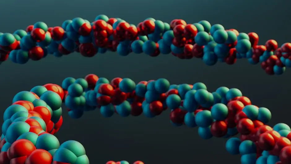
Unlock the secrets of protein evolution and function by mastering hierarchical clustering in R. Proteins, the workhorses of life, orchestrate nearly every biological process. Grouping them by sequence similarity is not merely a computational exercise; it's a strategic move to infer functional relationships, predict structural motifs, and trace evolutionary lineages. Imagine forging a path through a dense biological forest, identifying families and sub-families of proteins that share a common ancestry or perform similar tasks. This article activates your capabilities to achieve just that, transforming raw sequence data into actionable biological intelligence.

We will engineer a robust bioinformatics pipeline using R, guiding you from data preparation through advanced clustering techniques. Dive deep into the methodologies that allow us to organize diverse protein sequences into coherent, biologically meaningful groups. This exploration empowers you to accelerate your research, streamline drug discovery efforts, or simply gain a profound understanding of protein diversity. Prepare to revolutionize your approach to
decoding complex biological datasets with R for insightful statistical analysis, compelling visualization, and robust inference, embarking on a journey to uncover the hidden kinship among proteins.

Published on: 26 September 2026

Forge Protein Insights: Understanding Hierarchical Clustering Foundations

Hierarchical clustering stands as a cornerstone method for discerning natural groupings within protein sequences. This technique constructs a hierarchy of clusters, represented visually as a dendrogram, which reflects the varying degrees of similarity between proteins. Unlike flat clustering methods like k-means, hierarchical approaches do not necessitate a predefined number of clusters, offering a more exploratory path to uncover relationships. We will employ an agglomerative strategy, beginning with each protein as its own cluster and progressively merging the most similar clusters until all proteins reside within a single, encompassing cluster.

The journey commences with meticulous data preparation. Protein sequences, typically obtained from databases in FASTA format, demand careful handling. Ensure your sequences are clean, free from spurious characters, and correctly translated. The R packages Biostrings and DECIPHER provide robust functionalities for importing, manipulating, and analyzing biological sequence data. Biostrings, part of Bioconductor, offers specialized classes like AAStringSet for efficient storage and operations on amino acid sequences, acting as our foundational data structure. Preparing these sequences accurately establishes the bedrock for all subsequent analytical steps, ensuring the integrity and reliability of our clustering outcomes.

if (!requireNamespace("BiocManager", quietly = TRUE)) {
    install.packages("BiocManager")
}
BiocManager::install(c("Biostrings", "DECIPHER"))

library(Biostrings)
library(DECIPHER)

# --- Step 1: Prepare Protein Sequences ---
# For demonstration, we'll create a small set of dummy protein sequences.
# In a real scenario, you would read sequences from a FASTA file.
# Example: sequences <- readAAStringSet("your_proteins.fasta")

protein_data <- c(
    "P1" = "MALWMRLLPLLALLALWGPDPAAAFVNQHLCGSHLVEALYLVCGERGFFYTPKTRREAEDLQVGQVELGGGPGAGSLQPLALEGSLQKRGIVEQCCTSI CSLYQLENYCN",
    "P2" = "MALWMRLLPLLALLALWGPDPAAAFVNQHLCGSHLVEALYLVCGERGFFYTPKTRREAEDLQVGQVELGGGPGAGSLQPLALEGSLQKRGIVEQCCTSI CSLYQLENYCN",
    "P3" = "MALWMRLLPLLALLALWGPDPAAAFVNQHLCGSHLVEALYLVCGERGFFYTPKTRREAEDLQVGQVELGGGPGAGSLQPLALEGSLQKRGIVEQCCTSI CSLYQLENYCN",
    "P4" = "MKGLWPRLLPALVLAAALGAPDAAVVVNNQLCGARLVEALYLVGGERSFFYCPKTRREADDLQWGQVELGGGPGAGSLQALALRGSFQARGIVEQCCTSI CSLYQLENYCG",
    "P5" = "MALWPRLLPALVLAAALGAPDAAVVVNNQLCGARLVEALYLVGGERSFFYCPKTRREADDLQWGQVELGGGPGAGSLQALALRGSFQARGIVEQCCTSI CSLYQLENYCG",
    "P6" = "MGGRGLGLGLLGLLLLLLWLLQGDVGSKGRQLAALAEARLRLHWDNLRNLFLALLALLQGFLEGRRGNLRGNGLLLRGLPQLAAARLAAEQGRGLLGRGNLG",
    "P7" = "MGGRGLGLGLLGLLLLLLWLLQGDVGSKGRQLAALAEARLRLHWDNLRNLFLALLALLQGFLEGRRGNLRGNGLLLRGLPQLAAARLAAEQGRGLLGRGNLG",
    "P8" = "MSGRGVGLGLLGLLLLLLWLLQGDVGSKGRQLAALAEARLRLHWDNLRNLFLALLALLQGFLEGRRGNLRGNGLLLRGLPQLAAARLAAEQGRGLLGRGNLG"
)

# Convert to AAStringSet object, which Biostrings and DECIPHER functions expect.
sequences <- AAStringSet(protein_data)
names(sequences) <- names(protein_data)

print("Protein sequences loaded successfully:")
print(sequences)

Activate Similarity: Calculating Protein Distance Matrices

Quantifying the relatedness between protein sequences is the pivotal step before clustering. This involves converting sequence similarity into a measurable distance or dissimilarity. The most reliable method hinges on pairwise sequence alignment, where optimal matches and mismatches are scored based on biologically informed substitution matrices. DECIPHER's AlignSeqs function executes robust multiple sequence alignments, which are crucial as a precursor to accurate distance calculations. This alignment reveals conserved regions and evolutionary insertions/deletions, providing the context for assessing similarity.

Following alignment, we activate similarity by generating a distance matrix. Each entry in this matrix represents the dissimilarity between a pair of proteins. For proteins, the choice of substitution matrix — such as BLOSUM62 or PAM250 — is paramount. BLOSUM62, for instance, is highly effective for moderately divergent sequences, reflecting biologically probable amino acid exchanges. The Distances function within DECIPHER elegantly translates alignment scores into a distance value, creating a symmetric matrix where higher values denote greater dissimilarity. This matrix then serves as the direct input for the hierarchical clustering algorithm, ensuring that our groupings are founded on precise, quantitative measures of protein relatedness.

library(Biostrings)
library(DECIPHER)

# --- Step 2: Perform Multiple Sequence Alignment (MSA) ---
# AlignSeqs function from DECIPHER package is powerful for protein alignment.
# It can be computationally intensive for very large datasets.
# For a small set, it's efficient.

aligned_sequences <- AlignSeqs(sequences, type = "protein", processors = NULL) # Use NULL for auto-detection or specify core count

print("Aligned protein sequences:")
print(aligned_sequences)

# --- Step 3: Calculate Distance Matrix ---
# Distances function calculates pairwise distances based on alignment.
# `method = "myers"` (Myers-Miller algorithm) is suitable for protein sequences.
# `substitutionMatrix` can be BLOSUM62 (default), BLOSUM50, PAM250 etc.
# `correction = "jukes-cantor"` or `"kimura"` are typically for DNA, for proteins a direct score-to-distance conversion is more common.
# Here, `type = "matrix"` returns a matrix directly.

dist_matrix <- Distances(aligned_sequences,
                         type = "matrix",
                         method = "divergence", # Divergence directly from aligned sequences is common for protein distances
                         correction = NULL,    # No phylogenetic correction needed here for simple distance for clustering
                         substitutionMatrix = "BLOSUM62", # Common choice for protein similarity
                         includeTerminalGaps = TRUE)

print("Protein Distance Matrix:")
print(round(dist_matrix, 3))

Engineer Kinship Trees: Applying Hierarchical Clustering in R

With the distance matrix meticulously computed, we are primed to engineer the kinship tree through hierarchical clustering. The core R function for this task is hclust(), which takes a distance object (converted from our distance matrix using as.dist()) and a specified linkage method. The choice of linkage method profoundly influences the shape and interpretation of your dendrogram. Common methods include:

Complete linkage: Merges clusters based on the maximum distance between their most distant members.
Average linkage (UPGMA): Considers the average distance between all pairs of members from the two clusters.
Single linkage: Based on the minimum distance between any two members of the clusters, prone to 'chaining'.
Ward's method (ward.D2): Minimizes the total within-cluster variance, often producing more compact, spherical clusters.

We typically initiate clustering with 'average' or 'ward.D2' for protein sequences, as they often yield biologically intuitive groupings. Executing hclust() generates a hierarchical clustering object. Visualizing this object as a dendrogram is crucial. The dendrogram's branches represent clusters, and the height at which branches merge indicates the dissimilarity between those merged clusters. Taller branches signify greater divergence. By carefully examining this visual output, we can begin to discern distinct protein families and sub-families, solidifying our understanding of their kinship.

library(Biostrings)
library(DECIPHER)

# Assuming 'dist_matrix' is already computed from the previous step
# If starting fresh or rerunning:
# protein_data <- c(...)
# sequences <- AAStringSet(protein_data)
# aligned_sequences <- AlignSeqs(sequences, type = "protein", processors = NULL)
# dist_matrix <- Distances(aligned_sequences, type = "matrix", method = "divergence", substitutionMatrix = "BLOSUM62", includeTerminalGaps = TRUE)

# --- Step 4: Perform Hierarchical Clustering ---
# `hclust` function takes a distance object (as produced by `as.dist`) or a symmetric matrix.
# Key linkage methods:
#   "complete": Maximum distance between any two points in the clusters.
#   "average": Average distance between all pairs of points in the clusters (UPGMA).
#   "single": Minimum distance between any two points in the clusters.
#   "ward.D2": Minimizes the total within-cluster variance.

hc_result <- hclust(as.dist(dist_matrix), method = "average")

print("Hierarchical Clustering Result (hclust object):")
print(hc_result)

# --- Step 5: Visualize the Dendrogram ---
# Plot the dendrogram using base R graphics.
# This visualizes the hierarchy of clusters.

plot(hc_result,
     main = "Protein Sequence Hierarchical Clustering Dendrogram",
     xlab = "Protein ID",
     ylab = "Distance",
     hang = -1, # Aligns labels at the bottom
     cex = 0.8) # Adjust label size

# Add a horizontal line to indicate a potential cut-off for clusters
# Example: cut at a distance of 0.2
# abline(h = 0.2, col = "red", lty = 2)

Optimize Discovery: Interpreting Protein Clusters and Validation

The ultimate goal of hierarchical clustering is not merely to build a dendrogram, but to optimize discovery by interpreting the resulting protein clusters in a biologically meaningful context. After generating the dendrogram, the next critical step involves 'cutting' it to define discrete clusters. The cutree() function in R allows you to specify either a desired number of clusters (k) or a specific height (h) on the dendrogram to make the cut. The choice of k or h often involves a blend of visual inspection, domain expertise, and, for larger datasets, objective metrics.

Once clusters are assigned, a rigorous validation process is essential. We must question whether these clusters represent true biological distinctions – do proteins within a cluster share common functional domains, active sites, or participate in the same pathways? This external validation, leveraging existing biological knowledge or experimental data, is paramount. Internal validation metrics, such as silhouette width (available in the cluster package), can provide a quantitative measure of how well each protein fits into its assigned cluster versus neighboring clusters. Common pitfalls include choosing an inappropriate distance metric, selecting an arbitrary cut-off height without biological justification, or misinterpreting dendrogram branches. By combining computational rigor with biological insight, we transform raw sequence data into profound insights into protein function and evolution.

library(Biostrings)
library(DECIPHER)

# Assuming 'hc_result' is already computed from the previous step.
# If starting fresh or rerunning:
# ... (previous code for sequences, alignment, dist_matrix, hc_result)

# --- Step 6: Extract Clusters from the Dendrogram ---
# `cutree` function allows cutting the dendrogram to obtain clusters.
# You can specify either the number of clusters (k) or a height (h) to cut.
# Let's aim for 3 clusters based on visual inspection of the example dendrogram.

num_clusters <- 3 # Or choose based on biological knowledge or dendrogram inspection
protein_clusters <- cutree(hc_result, k = num_clusters)

print(paste("Number of clusters identified:", max(protein_clusters)))
print("Protein IDs and their cluster assignments:")
print(protein_clusters)

# --- Step 7: Analyze and Visualize Clusters (Example: Tabulate and simple plot) ---
# You can further analyze each cluster. For example, by extracting sequences,
# finding common motifs, or mapping known functional annotations.

# Convert cluster assignments to a data frame for easier manipulation
cluster_df <- data.frame(ProteinID = names(protein_clusters),
                           Cluster = as.factor(protein_clusters))

print("Cluster distribution:")
print(table(cluster_df$Cluster))

# Optional: Visualize specific cluster properties
# For real data, you might align clusters separately, compute physicochemical properties,
# or integrate with external functional annotation data (e.g., Gene Ontology).

# A simple plot of cluster members (conceptual, requires more complex data for real insights)
# This is a placeholder for demonstrating how to use cluster assignments.

# Example of how you might further process clusters:
for (i in 1:num_clusters) {
    cluster_members <- names(protein_clusters[protein_clusters == i])
    print(paste0("Cluster ", i, " members: ", paste(cluster_members, collapse = ", ")))
    # Example: Retrieve sequences for this cluster
    # cluster_seqs <- sequences[cluster_members]
    # Further analysis on cluster_seqs (e.g., motif discovery, functional enrichment)
}

# --- Step 8: Validation (Conceptual Discussion) ---
# For validation, one might use internal metrics like silhouette width (from `cluster` package)
# or external validation against known protein families/functions.
# Biologically, inspect if clustered proteins share domains, active sites, or pathways.

# Example of silhouette calculation (requires the 'cluster' package)
# library(cluster)
# silhouette_scores <- silhouette(protein_clusters, as.dist(dist_matrix))
# plot(silhouette_scores)
# summary(silhouette_scores)

Key Takeaways

Hierarchical Clustering: A Strategic Tool for Protein Analysis

Hierarchical clustering organizes protein sequences based on similarity, revealing evolutionary relationships and functional groups. Unlike k-means, it doesn't require a predefined number of clusters, making it ideal for exploratory analyses. The process builds a dendrogram, a tree-like diagram visualizing the hierarchy of clusters, crucial for inferring protein kinship.

Data Preparation and Sequence Alignment are Critical

The foundation of accurate protein clustering lies in meticulous data preparation. Sequences, typically in FASTA format, must be cleaned and converted into appropriate R objects (e.g., AAStringSet using Biostrings). Subsequent multiple sequence alignment (MSA) using tools like DECIPHER's AlignSeqs is paramount. MSA identifies conserved regions and provides the context for quantifying true biological similarity, preventing misinterpretations from raw sequence comparisons.

Distance Matrix Quantifies Protein Relatedness

After alignment, calculating a distance matrix is the next vital step. This matrix quantifies the dissimilarity between all pairs of proteins. The choice of substitution matrix (e.g., BLOSUM62 for divergent proteins) is crucial for translating alignment scores into meaningful biological distances. DECIPHER's Distances function robustly computes this matrix, which serves as the direct input for the clustering algorithm.

`hclust()` and Linkage Methods Drive Cluster Formation

The R function hclust() is the core of hierarchical clustering. It takes the distance matrix and a chosen linkage method (e.g., 'average', 'complete', 'ward.D2'). Linkage methods dictate how distances between clusters are measured, significantly influencing the dendrogram's structure. 'Average' and 'ward.D2' are often preferred for protein data due to their balance in forming cohesive clusters.

Interpreting and Validating Clusters is Key to Discovery

The ultimate value of clustering emerges from interpreting the dendrogram and extracting meaningful clusters using cutree(). The 'correct' number of clusters is often determined by a combination of visual inspection, biological context, and internal validation metrics (e.g., silhouette width). Clusters must be validated against existing biological knowledge (functional annotations, domains) to ensure their relevance and prevent misinterpretation of computational groupings as true biological insights.

Editorial Team

← Engineer Robustness: Clean & Normalize Protein Data in R Engineer Protein Similarity Heatmaps in R for Bio-Insights →

FAQ

Why choose hierarchical clustering over K-means for protein sequences?

Hierarchical clustering is often preferred for protein sequences because it does not require pre-specifying the number of clusters (k), which is rarely known in advance for biological data. It provides a visual dendrogram, allowing for intuitive exploration of relationships at different levels of similarity, revealing evolutionary histories and subtle sub-groupings. K-means, while faster for very large datasets, forces a fixed number of clusters and doesn't inherently reveal the nested relationships crucial for understanding protein families.
How do I choose the optimal distance metric and linkage method for protein clustering?

Choosing the distance metric is critical; for proteins, it typically stems from pairwise sequence alignment using biologically informed substitution matrices like BLOSUM62 (for more divergent sequences) or PAM (for closely related ones). The 'divergence' method in DECIPHER is robust. For linkage, 'average' (UPGMA) is a common default, balancing cluster size and distance. 'Ward.D2' can create more compact, equally sized clusters. The 'best' choice is often empirically determined, comparing results with known biological groupings or using internal validation metrics like silhouette scores.
How can I determine the 'correct' number of protein clusters from a dendrogram?

Determining the 'correct' number of clusters is often a blend of art and science. Visually, look for long horizontal lines indicating large distance gaps before clusters merge, suggesting natural breaks. Biologically, refer to existing knowledge about protein families or domains; does a cut-off yield groups consistent with known functions? Mathematically, methods like the silhouette plot, gap statistic, or elbow method (though less direct for hierarchical) can suggest an optimal number. Ultimately, the most insightful number of clusters will be one that maximizes biological interpretability and relevance to your research question.
What are common pitfalls or challenges when clustering protein sequences?

Common challenges include handling very large datasets (computational cost), sensitivity to the chosen distance metric and linkage method, and the presence of highly divergent sequences or outliers that can distort cluster structures. Misinterpreting the dendrogram's height or branches, or assuming all clusters are equally biologically significant, are also pitfalls. Ensuring high-quality sequence alignment, validating clusters with external biological data, and iteratively experimenting with different parameters are best practices to mitigate these issues.
Are there R packages beyond Biostrings and DECIPHER useful for protein clustering?

Absolutely. While Biostrings and DECIPHER are foundational for sequence handling and alignment, other packages enhance the pipeline. ape (Analyses of Phylogenetics and Evolution) is excellent for visualizing phylogenetic trees and manipulating tree objects. ggdendro extends dendrogram visualization with ggplot2 for publication-quality graphics. For internal cluster validation, the cluster package offers metrics like silhouette width. These packages collectively empower a comprehensive and visually rich protein clustering workflow in R.

Statistical Analysis in R