
> Bio-engineering & bioinformatics pipelines > Statistical Analysis in R > Engineer Automated R Pipelines for Batch Protein Analysis
Engineer Automated R Pipelines for Batch Protein Analysis
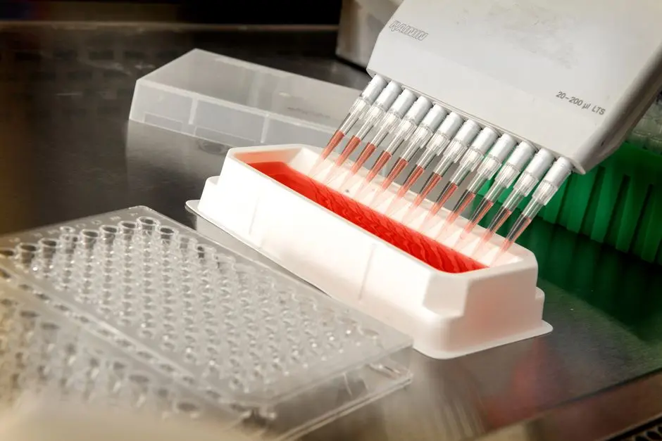
Unlock unparalleled efficiency in your proteomic research. We confront the inherent challenge of processing vast, multi-batch protein datasets—a task traditionally consuming critical time and prone to manual error. This resource empowers you to transform repetitive analytical chores into streamlined, automated workflows using R scripting. We illuminate a strategic pathway, guiding you to forge robust pipelines that consistently deliver accurate, high-fidelity statistical insights. Prepare to master techniques that not only accelerate your data processing but also elevate the reproducibility and integrity of your scientific findings. Discover how to decipher biological datasets using R for robust statistical analysis, insightful visualization, and powerful inference, liberating your focus for deeper scientific inquiry rather than tedious data manipulation. This guide equips you with the tools to conquer complex proteomic landscapes, ensuring every dataset yields its full story with precision and speed.
Forge Robust R Pipelines: Blueprinting Your Automation Strategy
We initiate the journey by establishing a robust foundation for our R automation pipeline. This critical first step involves meticulously blueprinting our environment, ensuring all necessary computational scaffolding is in place. We activate essential R packages, such as tidyverse for its comprehensive suite of data manipulation and visualization tools, data.table for its unparalleled efficiency in handling large datasets, and readxl for seamless ingestion of Excel files. Prioritize this setup; a well-configured environment prevents countless downstream errors.
Next, we engineer a logical and hierarchical project structure. This isn't merely organizational; it's a strategic imperative for maintainability, reproducibility, and collaborative efforts. Establish dedicated directories for raw data, processed outputs, analysis scripts, and final results (tables, plots). This clear separation prevents data entanglement and facilitates rapid navigation, especially when managing dozens of datasets. Implement version control from the outset; Git, for instance, safeguards your evolving code and tracks every modification, a non-negotiable practice in scientific computing. We systematically create these directories, hardening our project's resilience against disorganization. This proactive structuring minimizes cognitive load and maximizes focus on the core biological questions, transforming a potential chaotic mess into an ordered scientific workspace.
# 1. Install necessary packages if not already installed
install.packages(c("tidyverse", "data.table", "readxl"))

# 2. Load required libraries
library(tidyverse)    # For data manipulation (dplyr, ggplot2, etc.)
library(data.table)   # For efficient data handling, especially large datasets
library(readxl)       # For reading .xlsx files

# 3. Define the base directory where your datasets are located
# IMPORTANT: Replace 'path/to/your/protein/data' with your actual directory path
base_data_dir <- "path/to/your/protein/data"

# 4. Create a consistent project structure (optional but highly recommended)
# This helps organize raw data, scripts, and output files.
project_structure_paths <- c(
  file.path(base_data_dir, "raw_data"),
  file.path(base_data_dir, "processed_data"),
  file.path(base_data_dir, "scripts"),
  file.path(base_data_dir, "results", "tables"),
  file.path(base_data_dir, "results", "plots")
)

# Check if directories exist and create them if not
for (path in project_structure_paths) {
  if (!dir.exists(path)) {
    dir.create(path, recursive = TRUE)
    cat(paste0("Created directory: ", path, "\n"))
  } else {
    cat(paste0("Directory already exists: ", path, "\n"))
  }
}

# Example: Create dummy data files for demonstration
# In a real scenario, these would be your actual protein datasets
set.seed(123)
for (i in 1:3) {
  df <- data.frame(
    Protein_ID = paste0("P", 1:100),
    Sample_A = rnorm(100, mean = 10, sd = 2),
    Sample_B = rnorm(100, mean = 12, sd = 2),
    Sample_C = rnorm(100, mean = 10, sd = 2)
  )
  write.csv(df, file.path(base_data_dir, "raw_data", paste0("dataset_", i, ".csv")), row.names = FALSE)
}
cat(paste0("Created 3 dummy datasets in: ", file.path(base_data_dir, "raw_data"), "\n"))
Activate Data Ingestion & Preprocessing: Engineering Harmonized Datasets
We activate the core engine of our pipeline: robust data ingestion and preprocessing. This phase is paramount; the quality of your insights directly correlates with the quality and consistency of your input data. We engineer a specialized R function designed to handle diverse file formats—CSV, Excel, and potentially others—ensuring flexible adaptability to varying data sources. This function will systematically load each protein dataset, extract crucial metadata like the dataset's origin, and impose a standardized structure. This harmonization is critical, as inconsistencies in column names, data types, or missing value representations can derail an entire analysis.
Within this function, we rigorously address common data quality issues. We enforce the presence of essential identifiers, such as 'Protein_ID', preventing analysis failures due to malformed inputs. Furthermore, we implement intelligent strategies for handling missing values (NAs). While a simplistic approach might replace NAs with zero, a more nuanced strategy involves imputation based on experimental context or statistical methods. We transform relevant columns into appropriate numeric types, ensuring all downstream statistical operations are valid. This meticulous preprocessing ensures that every dataset, regardless of its original format, emerges clean, consistent, and ready for advanced statistical interrogation. This disciplined approach builds a reliable analytical foundation, mitigating the risk of misleading results.
# 1. Define a function to load and preprocess a single protein dataset
# This function takes the file path of a dataset as input.
preprocess_protein_data <- function(file_path) {

  # Extract dataset name from file_path (e.g., 'dataset_1')
  dataset_name <- tools::file_path_sans_ext(basename(file_path))

  # Determine file type and read data accordingly
  if (grepl("\.csv$", file_path, ignore.case = TRUE)) {
    df <- read.csv(file_path, stringsAsFactors = FALSE)
  } else if (grepl("\.xlsx?$", file_path, ignore.case = TRUE)) {
    df <- read_excel(file_path) # Assumes first sheet by default
  } else {
    stop(paste0("Unsupported file type for: ", file_path, ". Please use .csv or .xlsx."))
  }

  # Ensure 'Protein_ID' column exists
  if (!"Protein_ID" %in% names(df)) {
    stop(paste0("Missing 'Protein_ID' column in dataset: ", dataset_name))
  }

  # Convert to data.table for efficient manipulation
  setDT(df)

  # Perform basic preprocessing:
  # - Convert relevant columns to numeric (excluding Protein_ID)
  numeric_cols <- setdiff(names(df), "Protein_ID")
  df[, (numeric_cols) := lapply(.SD, as.numeric), .SDcols = numeric_cols]

  # - Handle missing values (example: replace with 0 or mean, or impute)
  # For demonstration, we'll replace NA with 0. Adapt this strategy based on your data and research question.
  # Common error: blindly replacing NA. Understand its origin before imputation.
  df[is.na(df)] <- 0 # IMPORTANT: Customize NA handling strategy based on context

  # Add a 'Dataset_Source' column for traceability
  df[, Dataset_Source := dataset_name]

  return(df)
}

# 2. List all data files in the raw_data directory
# IMPORTANT: Ensure 'base_data_dir' is set correctly from the previous step
raw_data_path <- file.path(base_data_dir, "raw_data")
all_data_files <- list.files(raw_data_path, pattern = "\\.(csv|xlsx)$", full.names = TRUE, ignore.case = TRUE)

# Check if any files were found
if (length(all_data_files) == 0) {
  stop(paste0("No protein data files found in: ", raw_data_path, ". Please ensure your raw data is placed there."))
}

cat(paste0("Found ", length(all_data_files), " data files.\n"))

# 3. Apply the preprocessing function to all files
# This creates a list of preprocessed data tables.
preprocessed_datasets_list <- lapply(all_data_files, preprocess_protein_data)

# 4. (Optional) Combine all preprocessed datasets into a single large data.table
# This can be useful for global analysis or if you need to compare across all datasets in one go.
combined_protein_data <- rbindlist(preprocessed_datasets_list, fill = TRUE)

# Display structure of one preprocessed dataset and the combined data
cat("\nStructure of a sample preprocessed dataset:\n")
print(str(preprocessed_datasets_list[[1]]))

cat("\nHead of combined protein data (first 5 rows):\n")
print(head(combined_protein_data))
Decode Statistical Insights: Architecting the Analysis Engine
We decode the inherent biological signals by architecting a powerful statistical analysis engine. This involves crafting a modular R function, the analytical core, which accepts a single, preprocessed dataset and systematically extracts meaningful insights. Within this function, we embed standard statistical procedures essential for protein analysis, such as calculating log2 fold changes (Log2FC) to quantify the magnitude of protein abundance shifts between experimental conditions. We then activate robust inferential tests, typically Welch's t-test for comparing two groups or ANOVA for multiple groups, to assess the statistical significance of observed differences.
Crucially, our engine incorporates mechanisms for multiple hypothesis correction. Running numerous statistical tests (one per protein) dramatically inflates the false discovery rate. Therefore, we integrate methods like the Benjamini-Hochberg (BH) procedure to adjust p-values, ensuring that reported significances are statistically rigorous and reliable. This prevents us from erroneously identifying non-existent biological effects. The function concludes by flagging proteins that meet predefined criteria for both statistical significance (e.g., adjusted p-value < 0.05) and biological relevance (e.g., |Log2FC| > 1.5). Common errors include neglecting p-value adjustment or using arbitrary thresholds; our engineered solution systematically avoids these pitfalls, delivering high-confidence results. This modular design makes the analysis engine reusable and adaptable across diverse proteomic studies, maximizing its utility.
# 1. Define a core function for statistical analysis on a single preprocessed dataset
# This function performs differential expression analysis (e.g., t-test) and calculates fold changes.
perform_statistical_analysis <- function(dataset_dt, dataset_name) {

  # Ensure 'Protein_ID' and at least two numeric sample columns are present
  if (!"Protein_ID" %in% names(dataset_dt) || ncol(dataset_dt) < 3) {
    warning(paste0("Skipping analysis for ", dataset_name, ": Insufficient columns or missing Protein_ID."))
    return(NULL)
  }

  # Identify sample columns (assuming all numeric columns except Protein_ID and Dataset_Source are samples)
  sample_cols <- names(dataset_dt)[sapply(dataset_dt, is.numeric) & !names(dataset_dt) %in% c("Protein_ID", "Dataset_Source")]

  # For a simple differential analysis, we need at least two groups. Let's assume 'Sample_A' and 'Sample_B' for demonstration.
  # Adapt this based on your actual experimental design and column names.
  if (!all(c("Sample_A", "Sample_B") %in% sample_cols)) {
    warning(paste0("Skipping differential analysis for ", dataset_name, ": 'Sample_A' or 'Sample_B' not found."))
    return(NULL)
  }

  # Initialize an empty list to store results for this dataset
  results_list <- list()

  # Calculate Log2 Fold Change (LF2C) for Sample_B vs Sample_A
  # Add a small pseudo-count (e.g., 1) to avoid log2(0) if data can be 0
  dataset_dt[, Log2FC := log2((Sample_B + 1) / (Sample_A + 1))]

  # Perform Welch's t-test for each protein (comparing Sample_A vs Sample_B)
  # Using `map` from `purrr` (part of tidyverse) for functional programming
  t_test_results <- dataset_dt %>%
    group_by(Protein_ID) %>%
    summarise(
      P_value = tryCatch({
        t_test <- t.test(Sample_B, Sample_A, var.equal = FALSE) # Welch's t-test
        t_test$p.value
      }, error = function(e) NA_real_) # Handle cases where t-test might fail (e.g., all values are same)
    ) %>%
    ungroup()

  # Merge t-test results back with the main dataset_dt
  dataset_dt <- merge(dataset_dt, t_test_results, by = "Protein_ID", all.x = TRUE)

  # Adjust p-values for multiple comparisons (e.g., Benjamini-Hochberg)
  dataset_dt[, Adjusted_P_value := p.adjust(P_value, method = "BH")]

  # Flag differentially expressed proteins (example thresholds)
  dataset_dt[, Is_DE := Adjusted_P_value < 0.05 & abs(Log2FC) > log2(1.5)] # Fold change > 1.5 or < 1/1.5

  # Store results for this dataset
  results_list$summary_stats <- dataset_dt
  results_list$name <- dataset_name

  return(results_list)
}

# Example: Apply the analysis function to one of the preprocessed datasets
# Assuming 'preprocessed_datasets_list' and 'combined_protein_data' from previous step are available
if (length(preprocessed_datasets_list) > 0) {
  cat("\nRunning analysis on the first preprocessed dataset as an example:\n")
  example_analysis_output <- perform_statistical_analysis(preprocessed_datasets_list[[1]], preprocessed_datasets_list[[1]]$Dataset_Source[1])

  if (!is.null(example_analysis_output)) {
    cat("\nHead of analysis results for the example dataset:\n")
    print(head(example_analysis_output$summary_stats))

    cat("\nNumber of differentially expressed proteins in example dataset:\n")
    print(sum(example_analysis_output$summary_stats$Is_DE, na.rm = TRUE))
  }
} else {
  cat("No preprocessed datasets available for example analysis.\n")
}
Engineer Batch Processing Mastery: Deploying Automated Workflows
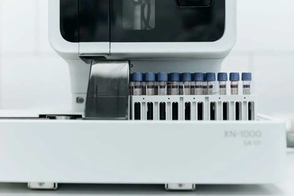
We engineer batch processing mastery, deploying automated workflows that liberate us from repetitive manual execution. This stage orchestrates the seamless application of our previously defined preprocessing and statistical analysis functions across every dataset in our designated directory. We primarily leverage a for loop or functional programming constructs like lapply or purrr::map to iterate through a list of file paths. Each iteration invokes the entire analytical sequence for a single dataset, ensuring uniformity and minimizing human error. This systematic approach is the cornerstone of high-throughput biology.
A critical component of robust batch processing is intelligent error handling. We integrate tryCatch blocks around our processing functions. This strategic inclusion ensures that if an individual dataset encounters an anomaly (e.g., malformed data, missing columns), the pipeline gracefully logs the error without crashing the entire operation. This allows the process to continue with subsequent datasets, maximizing throughput and providing clear diagnostics for later review. After each dataset's analysis completes, we systematically store its results—be it summary statistics, differentially expressed protein lists, or generated plots—in a structured manner. This consolidated storage facilitates later aggregation and comprehensive reporting, turning a multitude of individual analyses into a unified, actionable scientific narrative. We ensure maximum resilience and uninterrupted data flow, even in the face of imperfect data.
# 1. Collect all raw data files again (or use the list from preprocess step)
raw_data_path <- file.path(base_data_dir, "raw_data")
all_data_files <- list.files(raw_data_path, pattern = "\\.(csv|xlsx)$", full.names = TRUE, ignore.case = TRUE)

if (length(all_data_files) == 0) {
  stop(paste0("No data files found in ", raw_data_path, " to process."))
}

# 2. Initialize a list to store all analysis results from batch processing
all_batch_results <- list()

cat("\nInitiating batch processing across all datasets...\n")

# 3. Implement the batch processing loop
for (file_path in all_data_files) {

  dataset_id <- tools::file_path_sans_ext(basename(file_path))
  cat(paste0("  Processing dataset: ", dataset_id, "\n"))

  # Use tryCatch to gracefully handle errors in individual datasets
  # This prevents the entire pipeline from crashing if one file has issues.
  tryCatch({
    # Step A: Preprocess the current dataset
    current_preprocessed_data <- preprocess_protein_data(file_path)

    # Step B: Perform statistical analysis on the preprocessed data
    if (!is.null(current_preprocessed_data)) {
      analysis_output <- perform_statistical_analysis(current_preprocessed_data, dataset_id)

      # Store the results if analysis was successful
      if (!is.null(analysis_output)) {
        all_batch_results[[dataset_id]] <- analysis_output$summary_stats
        cat(paste0("    Analysis complete for ", dataset_id, ".\n"))
      } else {
        warning(paste0("    Analysis returned NULL for ", dataset_id, ". Skipping storage.\n"))
      }
    } else {
      warning(paste0("    Preprocessing returned NULL for ", dataset_id, ". Skipping analysis.\n"))
    }

  }, error = function(e) {
    cat(paste0("    ERROR processing ", dataset_id, ": ", e$message, "\n"))
    # Log the error for review, but continue with other datasets
  })
}

cat("Batch processing finished.\n")

# 4. (Optional) Inspect the collected batch results
# Example: Display names of datasets successfully analyzed
if (length(all_batch_results) > 0) {
  cat("\nSuccessfully analyzed datasets:\n")
  print(names(all_batch_results))

  # Example: Access results for a specific dataset
  # print(head(all_batch_results[["dataset_1"]]))
} else {
  cat("No datasets were successfully analyzed in the batch process.\n")
}
Optimize Reporting & Visualization: Consolidating Actionable Outcomes
We optimize reporting and visualization, consolidating raw analytical outputs into actionable scientific narratives. This final stage of the pipeline transforms complex data into accessible tables and compelling graphics, crucial for communicating discoveries. We systematically iterate through the results of each processed dataset, generating distinct output files. For every dataset, we save a detailed table containing all calculated statistics—Log2FC, p-values, adjusted p-values, and differential expression flags—ensuring full transparency and traceability of the findings. This archival step is paramount for long-term data integrity.
Simultaneously, we automate the generation of informative visualizations. A classic example in proteomics is the Volcano plot, which graphically depicts both the magnitude and statistical significance of protein changes, immediately highlighting potential biological candidates. Our pipeline engineers R scripts using ggplot2 to produce these plots, ensuring consistent aesthetics and annotations across all datasets. Furthermore, we activate the creation of concise summary reports for each dataset, outlining key metrics such as the total number of proteins analyzed and the count of differentially expressed proteins. These automated reports provide an immediate snapshot of each study's core findings. Finally, we synthesize these individual reports into a global overview, compiling all differentially expressed proteins from across the entire batch into a single master table. This comprehensive aggregation elevates individual findings into a broader, comparative biological context, maximizing the scientific leverage derived from the automated workflow.
# 1. Define output directories from the initial setup
results_tables_dir <- file.path(base_data_dir, "results", "tables")
results_plots_dir <- file.path(base_data_dir, "results", "plots")

# 2. Iterate through all batch results to generate reports and plots
cat("\nGenerating reports and visualizations...\n")

if (length(all_batch_results) == 0) {
  stop("No batch analysis results found to generate reports and plots from.")
}

for (dataset_name in names(all_batch_results)) {

  current_results_dt <- all_batch_results[[dataset_name]]
  cat(paste0("  Reporting for dataset: ", dataset_name, "\n"))

  # Step A: Save detailed results table for each dataset
  output_table_path <- file.path(results_tables_dir, paste0(dataset_name, "_analysis_results.csv"))
  write.csv(current_results_dt, output_table_path, row.names = FALSE)
  cat(paste0("    Saved results table to: ", output_table_path, "\n"))

  # Step B: Generate a Volcano Plot for differential expression visualization
  # Ensure ggplot2 is loaded (from tidyverse)
  if ("Log2FC" %in% names(current_results_dt) && "Adjusted_P_value" %in% names(current_results_dt)) {

    # For plotting, replace -log10(0) with a slightly larger value to avoid infinite values
    current_results_dt[, neg_log10_adj_p := -log10(Adjusted_P_value + .Machine$double.eps)]

    # Define colors for significantly expressed proteins
    volcano_plot <- ggplot(current_results_dt, aes(x = Log2FC, y = neg_log10_adj_p, color = Is_DE)) +
      geom_point(alpha = 0.6, size = 1.5) +
      scale_color_manual(values = c("FALSE" = "grey", "TRUE" = "red")) +
      geom_vline(xintercept = c(-log2(1.5), log2(1.5)), linetype = "dashed", color = "blue") +
      geom_hline(yintercept = -log10(0.05), linetype = "dashed", color = "blue") +
      labs(
        title = paste0("Volcano Plot for ", dataset_name),
        x = "Log2 Fold Change (Sample_B vs Sample_A)",
        y = "-log10(Adjusted P-value)"
      ) +
      theme_minimal() +
      theme(legend.position = "bottom", plot.title = element_text(hjust = 0.5))

    output_plot_path <- file.path(results_plots_dir, paste0(dataset_name, "_volcano_plot.png"))
    ggsave(output_plot_path, plot = volcano_plot, width = 8, height = 6, dpi = 300)
    cat(paste0("    Saved Volcano Plot to: ", output_plot_path, "\n"))

  } else {
    warning(paste0("    Skipping Volcano Plot for ", dataset_name, ": Missing 'Log2FC' or 'Adjusted_P_value' columns.\n"))
  }

  # Step C: Generate a summary report for each dataset (e.g., number of DE proteins)
  num_de_proteins <- sum(current_results_dt$Is_DE, na.rm = TRUE)
  total_proteins <- nrow(current_results_dt)

  summary_report_text <- paste0(
    "Analysis Summary for ", dataset_name, ":\n",
    "-----------------------------------------------------\n",
    "Total proteins analyzed: ", total_proteins, "\n",
    "Differentially expressed proteins (Adj P < 0.05, |Log2FC| > log2(1.5)): ", num_de_proteins, "\n",
    "Ratio of DE proteins: ", round(num_de_proteins / total_proteins * 100, 2), "%\n",
    "-----------------------------------------------------\n\n"
  )

  output_summary_path <- file.path(results_tables_dir, paste0(dataset_name, "_summary_report.txt"))
  writeLines(summary_report_text, output_summary_path)
  cat(paste0("    Saved summary report to: ", output_summary_path, "\n"))

}

cat("Reporting and visualization complete for all datasets.\n")

# 3. (Optional) Aggregate results across all datasets for a global overview
# Example: Create a master table of all DE proteins from all datasets
all_de_proteins_combined <- rbindlist(lapply(all_batch_results, function(dt) {
  dt[dt$Is_DE == TRUE, c("Protein_ID", "Log2FC", "Adjusted_P_value", "Dataset_Source"), with=FALSE]
}), fill = TRUE)

if (nrow(all_de_proteins_combined) > 0) {
  master_de_table_path <- file.path(results_tables_dir, "master_differentially_expressed_proteins.csv")
  write.csv(all_de_proteins_combined, master_de_table_path, row.names = FALSE)
  cat(paste0("\nSaved combined DE proteins to: ", master_de_table_path, "\n"))
  print(head(all_de_proteins_combined))
} else {
  cat("\nNo differentially expressed proteins found across all datasets for master table.\n")
}
Engineer Pipeline Resilience: Advanced Strategies for Bio-Computational Stability
We engineer pipeline resilience, deploying advanced strategies that harden our bio-computational workflows against failure and maximize efficiency. For substantial datasets or numerous batches, serial processing becomes a bottleneck. We conquer this limitation by activating parallelization. Leveraging packages like future.apply, we distribute analytical tasks across multiple CPU cores, dramatically accelerating processing times. This is not merely a speed boost; it is a strategic optimization that transforms weeks of computation into mere hours, enabling more iterative exploration and faster hypothesis testing. We carefully configure the number of parallel workers, balancing computational demand with system resources to ensure optimal performance without resource exhaustion.
Beyond speed, a resilient pipeline demands comprehensive visibility into its operations. We implement robust logging systems. Instead of merely printing messages to the console, our scripts record detailed execution logs—timestamps, processing status for each dataset, and specific error messages—to a dedicated file. This log acts as an invaluable diagnostic tool, allowing us to pinpoint the exact moment and cause of any failure without re-running the entire pipeline. It also serves as an audit trail, documenting the successful execution of each step. Furthermore, we embed rigorous validation checks at every stage: confirming file integrity, schema consistency, and statistical assumption adherence. These preemptive checks prevent erroneous data from propagating downstream, ensuring the unwavering quality of our scientific output. This meticulous attention to resilience transforms our automated pipelines into trustworthy, high-performance engines for biological discovery.
# 1. Install and load future.apply for parallel processing (if not already installed)
install.packages("future.apply")
library(future.apply) # For future_lapply

# 2. Configure a parallel processing strategy (e.g., using all but one core)
# IMPORTANT: Adjust 'workers' based on your system's capabilities and other tasks.
# For large number of small tasks, 'multisession' is good. For fewer large tasks, 'multicore' (Linux/macOS).
if (Sys.info()['sysname'] == 'Windows') {
  plan(multisession, workers = availableCores() - 1)
} else {
  plan(multicore, workers = availableCores() - 1)
}

cat(paste0("\nParallel processing activated with ", future::nbrOfWorkers(), " workers.\n"))

# 3. Modify the batch processing loop to use future_lapply for parallel execution
# This assumes preprocess_protein_data and perform_statistical_analysis are defined.

# Get the list of files again
raw_data_path <- file.path(base_data_dir, "raw_data")
all_data_files <- list.files(raw_data_path, pattern = "\\.(csv|xlsx)$", full.names = TRUE, ignore.case = TRUE)

if (length(all_data_files) == 0) {
  stop("No data files found to process in parallel.")
}

process_single_dataset_pipeline <- function(file_path) {
  dataset_id <- tools::file_path_sans_ext(basename(file_path))
  cat(paste0("  Processing dataset (worker): ", dataset_id, "\n"))

  result <- tryCatch({
    current_preprocessed_data <- preprocess_protein_data(file_path)
    if (!is.null(current_preprocessed_data)) {
      analysis_output <- perform_statistical_analysis(current_preprocessed_data, dataset_id)
      if (!is.null(analysis_output)) {
        return(analysis_output$summary_stats) # Return the summary stats data.table
      } else {
        warning(paste0("Analysis returned NULL for ", dataset_id, "."))
        return(NULL)
      }
    } else {
      warning(paste0("Preprocessing returned NULL for ", dataset_id, "."))
      return(NULL)
    }
  }, error = function(e) {
    warning(paste0("ERROR processing ", dataset_id, ": ", e$message))
    return(NULL)
  })
  return(list(dataset_id = dataset_id, result = result))
}

# Execute the pipeline in parallel
parallel_batch_results_list_of_lists <- future_lapply(all_data_files, process_single_dataset_pipeline)

# Convert results into a named list, filtering out NULLs
all_batch_results_parallel <- list()
for (res_item in parallel_batch_results_list_of_lists) {
  if (!is.null(res_item$result)) {
    all_batch_results_parallel[[res_item$dataset_id]] <- res_item$result
  }
}

cat("Parallel batch processing finished.\n")

# Display some results from parallel processing
if (length(all_batch_results_parallel) > 0) {
  cat("\nSuccessfully analyzed datasets in parallel:\n")
  print(names(all_batch_results_parallel))
  # The reporting and visualization steps would then use 'all_batch_results_parallel'
  # instead of 'all_batch_results'
} else {
  cat("No datasets were successfully analyzed in the parallel batch process.\n")
}

# 4. Implement a robust logging system (conceptual example)
# In a real pipeline, you would use a dedicated logging package (e.g., 'logger')
# This example just demonstrates writing messages to a log file.
log_file_path <- file.path(base_data_dir, "pipeline_log.txt")

# Function to append messages to log file
append_to_log <- function(message) {
  timestamp <- format(Sys.time(), "%Y-%m-%d %H:%M:%S")
  cat(paste0("[", timestamp, "] ", message, "\n"), file = log_file_path, append = TRUE)
}

# Example usage in the pipeline:
# append_to_log(paste0("Starting pipeline execution."))
# ... (after processing each dataset)
# append_to_log(paste0("Dataset '", dataset_id, "' processed successfully."))
# append_to_log(paste0("ERROR: Dataset '", dataset_id, "' failed with error: ", e$message))
# ...
# append_to_log(paste0("Pipeline execution finished."))
Key Takeaways
Strategic Pipeline Blueprinting
Establish a logical project structure with dedicated directories for raw data, scripts, and results. Prioritize installing and loading essential R packages (tidyverse, data.table, readxl) and implement version control early to ensure reproducibility and maintainability. A well-organized environment prevents chaos and streamlines complex workflows.
Robust Data Ingestion & Preprocessing
Engineer a modular R function to load and preprocess diverse data formats (CSV, Excel). This function must harmonize column names, enforce data types, and strategically handle missing values (NAs). This ensures consistent, clean data across all batches, forming a solid foundation for accurate statistical analysis and preventing downstream errors.
Architecting the Statistical Engine
Develop a core R function for performing statistical analysis on a single dataset. Include calculations for Log2 Fold Change (Log2FC), inferential tests (e.g., Welch's t-test), and crucial multiple hypothesis correction (e.g., Benjamini-Hochberg). Define clear thresholds for statistical significance and biological relevance to flag differentially expressed proteins. This modular engine is reusable and robust.
Mastering Batch Workflow Deployment
Implement an iterative mechanism (e.g., for loop, lapply, or future_lapply for parallel processing) to apply the preprocessing and analysis functions across all datasets. Integrate tryCatch for robust error handling, allowing the pipeline to continue even if individual datasets encounter issues. Systematically store results from each dataset for later aggregation.
Optimized Reporting & Visualization
Automate the generation of detailed result tables and insightful visualizations (e.g., Volcano plots) for each dataset using ggplot2. Consolidate key metrics into concise summary reports. Aggregate findings from all datasets into a master overview, transforming individual analyses into a unified, actionable scientific narrative.
Building Pipeline Resilience
Enhance pipeline robustness through parallelization (e.g., with future.apply) for speed, and implement comprehensive logging systems for diagnostics and audit trails. Integrate rigorous validation checks at each stage to ensure data integrity and prevent error propagation, establishing a trustworthy and high-performance analytical framework.
FAQ
-
Why is automating R scripts crucial for protein dataset analysis?
Automating R scripts is crucial because it significantly enhances efficiency, accuracy, and reproducibility. Manual analysis of multiple protein datasets is time-consuming, prone to human error, and inconsistent. Automation enables rapid, standardized processing across numerous datasets, freeing researchers to focus on biological interpretation rather than repetitive tasks. It guarantees that every dataset undergoes the exact same analytical steps, strengthening the integrity and comparability of your findings.
-
What are the common pitfalls in automating protein data analysis in R?
Common pitfalls include inconsistent data formats across datasets, inadequate error handling, neglecting multiple hypothesis correction, and a lack of clear project structure. Data harmonization is often underestimated; varying column names or data types will break a unified script. Without robust
tryCatchblocks, a single problematic file can halt the entire batch process. Ignoring p-value adjustments leads to inflated false positives. Finally, a disorganized project makes scripts difficult to maintain, share, and reproduce. -
How can I ensure the reproducibility of my automated R analysis pipeline?
To ensure reproducibility, implement strict version control (e.g., Git) for all scripts and configuration files. Document every step rigorously, including package versions used (e.g., with
renvorpackrat). Maintain a consistent project structure. Ensure all data preprocessing steps are explicit and automated. Use a seed for any random processes, and ideally, containerize your environment (e.g., Docker) to guarantee consistent dependencies across different computing environments. Your code must be runnable by others with minimal setup. -
What R packages are essential for building robust automation pipelines for protein data?
Essential packages include
tidyverse(fordplyrfor data manipulation,ggplot2for visualization),data.tablefor high-performance data handling,readxloropenxlsxfor Excel file import, andfsfor file system operations. For parallelization,future.applyorparallelare invaluable. For specialized proteomic analysis, consider packages likeDEPfor differential expression analysis orMSnbasefor mass spectrometry data, depending on your specific data type and analytical needs. A strong core foundation withtidyverseanddata.tableis often sufficient for general batch processing.