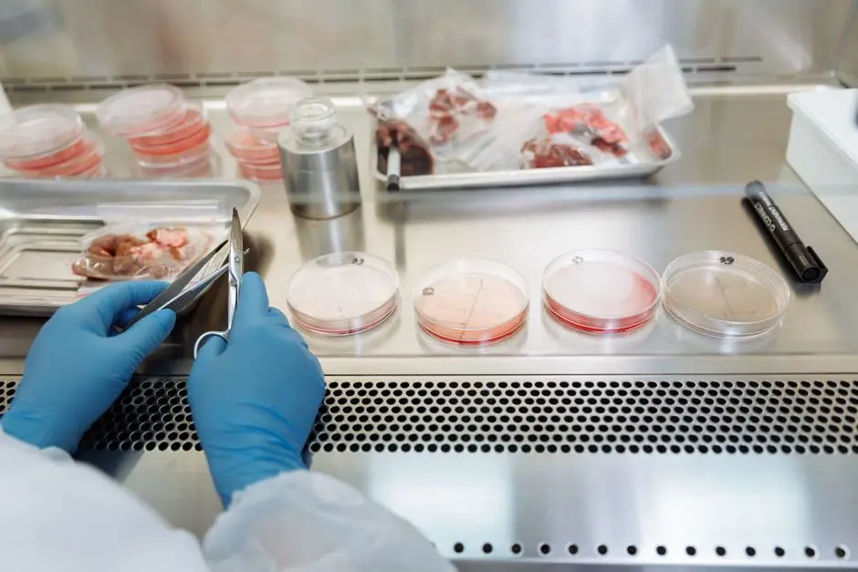
Every successful transcriptomics study commences long before the first sequencing read is generated, with meticulous experimental design and rigorous sample preparation. We must define our biological question precisely, then translate it into an experimental setup that yields statistically powerful and biologically meaningful data. Consider critical factors such as the number of biological replicates – a non-negotiable aspect to ensure statistical robustness and account for biological variability. For human studies, replicate counts of N=3-6 per group are often a minimum, while more complex designs might demand higher numbers. We also need to factor in potential batch effects, which can confound results; randomizing samples during processing and sequencing is a key mitigation strategy. Our sample collection protocols must be standardized, minimizing technical variation from the outset.

The integrity of RNA is paramount. We demand high-quality, intact RNA, as degradation profoundly biases downstream quantification. Utilize robust RNA extraction methods, tailored to your sample type, and meticulously assess RNA quality and quantity using tools like the Bioanalyzer or TapeStation. An RNA Integrity Number (RIN) or RNA Quality Number (RQN) > 8.0 is typically the gold standard, though some degraded samples (e.g., FFPE tissues) may necessitate specialized workflows. Following this, library preparation converts RNA into cDNA fragments suitable for sequencing, adding adapters and unique molecular identifiers (UMIs) if necessary, for multiplexing and removing PCR duplicates. Select a library prep kit appropriate for your RNA type (e.g., total RNA with ribosomal depletion vs. poly-A selection for mRNA) and research question. Neglecting these initial steps guarantees compromised results; precision here dictates the integrity of all subsequent analyses.

Upon receiving raw sequencing data, typically in FASTQ format, our immediate imperative is to establish data integrity and prepare it for downstream analysis. This phase is non-negotiable; compromised data quality yields unreliable biological insights. The initial step often involves demultiplexing, separating reads originating from different samples based on unique barcode sequences. Next, we rigorously assess read quality using tools like FastQC. This generates reports detailing per-base sequence quality, GC content, adapter contamination, and sequence duplication levels. We scrutinize these reports for deviations from expected distributions, which signal potential issues.

Armed with quality metrics, we proceed to trimming and filtering. Adapter sequences, low-quality bases (typically at the 3' end of reads), and short reads failing a minimum length threshold must be excised. Tools like Trimmomatic or FastP efficiently execute these tasks. This cleansing process is critical; retaining poor-quality data introduces noise and biases subsequent alignment and quantification. After trimming, we re-evaluate read quality to confirm improvements. The clean reads are then aligned to a reference genome or transcriptome using ultrafast and accurate aligners such as STAR or HISAT2. Crucially, these aligners must be aware of splice junctions to correctly map reads spanning exon boundaries. We generate alignment statistics – mapping rates, uniquely mapped reads, multimapped reads – which serve as further quality indicators. Low mapping rates can indicate poor sample quality, contamination, or a suboptimal reference genome. This rigorous architectural phase builds a solid foundation for gene expression quantification.

With high-quality, aligned reads, our next mission is to precisely quantify gene expression. The core task involves counting reads that map to annotated genes or transcripts. This step leverages genomic annotation files (GTF or GFF3) to define gene boundaries. Tools like featureCounts or HTSeq are industry standards, efficiently tallying reads for each feature (gene, exon, transcript). It’s crucial to understand how these tools handle ambiguously mapped reads or reads mapping to multiple features; consistent application is key. The output is typically a count matrix, where rows represent genes and columns represent samples, with each cell containing the raw read count for a given gene in a given sample.

Raw read counts, however, are not directly comparable across samples. They are influenced by sequencing depth (total number of reads per sample) and gene length (longer genes naturally accumulate more reads). Normalization is an indispensable step to remove these technical biases, enabling meaningful comparisons of gene expression levels. Early methods like RPKM (Reads Per Kilobase per Million mapped reads) and FPKM (Fragments Per Kilobase per Million mapped reads) attempted to normalize for both depth and length. However, for differential expression analysis, more sophisticated methods, such as those implemented in DESeq2 and edgeR, are preferred. These methods normalize for sequencing depth by estimating size factors that reflect library composition and apply statistical models robust to count data. TPM (Transcripts Per Million) offers a different approach, normalizing for gene length and sequencing depth, expressing gene abundance as a proportion of total transcripts. We must select the appropriate normalization strategy based on our downstream analysis goals; choosing correctly is vital for accurate interpretation.

Having quantified and normalized gene expression, we arrive at the pivotal stage: identifying biologically significant changes. Differential expression analysis (DEA) is our primary weapon, pinpointing genes whose expression levels significantly differ between experimental conditions (e.g., treatment vs. control, disease vs. healthy). Popular R packages like DESeq2 and edgeR employ statistical models specifically designed for RNA-seq count data, accounting for variance and dispersion. They output lists of differentially expressed genes (DEGs), typically ranked by p-value and fold-change. We establish significance thresholds, often a p-value < 0.05 combined with a false discovery rate (FDR) adjustment (e.g., Benjamini-Hochberg corrected p-value or adjusted p-value) and a minimum absolute log2 fold-change (e.g., > 1 or < -1), to minimize false positives and focus on robust changes.

Identifying DEGs is merely the first step; we must now interpret their biological meaning. Functional enrichment analysis deciphers the underlying biological processes, molecular functions, or cellular components associated with our DEG list. Tools like GOseq, DAVID, GSEA (Gene Set Enrichment Analysis), and IPA (Ingenuity Pathway Analysis) perform this by comparing our gene list against curated databases of biological pathways and ontologies. This reveals which pathways are activated or suppressed. Visualize these findings using heatmaps, volcano plots, and pathway diagrams to communicate the story effectively. Consider upstream regulator analysis to infer which transcription factors or microRNAs might be driving the observed gene expression changes. This holistic approach transforms raw data into a coherent narrative of biological function, forging a path from numerical counts to profound biological insight. We must always validate key findings with orthogonal methods, like qRT-PCR, to reinforce confidence in our conclusions.

We dissect the transcriptomics journey into five critical stages: 1. Experimental Design & Sample Prep: Define the question, ensure biological replicates (N≥3), standardize protocols, and achieve high RNA quality (RIN > 8.0). 2. Raw Data Processing & QC: Demultiplex, assess quality (FastQC), trim adapters/low-quality reads (Trimmomatic/FastP), and align to genome (STAR/HISAT2). 3. Quantification: Count reads per gene (featureCounts/HTSeq) to generate a raw count matrix. 4. Normalization: Adjust counts for sequencing depth and gene length, preferring methods like DESeq2/edgeR for differential expression. 5. Interpretation: Perform differential expression analysis (DESeq2/edgeR), identify DEGs, and conduct functional enrichment (GO/pathway analysis) to derive biological insights.

We leverage industry-standard tools: FastQC for quality assessment, Trimmomatic/FastP for read trimming, STAR/HISAT2 for alignment, featureCounts/HTSeq for read quantification, and DESeq2/edgeR for normalization and differential expression. Our best practices include: ensuring sufficient biological replicates, rigorously checking RNA integrity, minimizing batch effects through randomization, using appropriate normalization strategies, and validating key findings through orthogonal methods like qRT-PCR. We always interpret findings within a strong biological context and visualize results effectively to communicate complex data.