
> Computational Bio-Engineering & Molecular Coding > protein language models and transformers > Activate Biological Insights: UMAP Visualizations of Protein Embeddings
Activate Biological Insights: UMAP Visualizations of Protein Embeddings
Deciphering the intricate language of life demands advanced tools, especially when confronted with the deluge of high-dimensional data generated by modern biological experiments. Protein sequences, the fundamental blueprints of cellular function, now yield complex vector representations through powerful machine learning models. These vectors, known as biological embeddings, encode a wealth of information about protein structure, function, and evolutionary relationships. However, their high dimensionality—often hundreds or thousands of features—renders direct analysis and interpretation impossible. We stand at a critical juncture, needing to distill this complexity into actionable insights.
This resource engineers a robust code pipeline to conquer the 'curse of dimensionality,' transforming raw transformer vector dimensions into interpretable cluster distributions. We leverage UMAP (Uniform Manifold Approximation and Projection) to visualize these high-dimensional biological embeddings, revealing hidden patterns and structural families. UMAP empowers us to activate a deeper understanding of molecular relationships, guiding drug discovery, protein engineering, and fundamental biological research. Master this pipeline and unlock the latent biological leverage points embedded within your data. Explore the frontiers of Protein Language Models & Transformer Infrastructures and witness how sophisticated dimensionality reduction techniques become indispensable for scientific discovery.

Conquer High-Dimensionality: The Imperative for Biological Embedding Visualization
Biological embeddings forge a new frontier in understanding molecular biology. Protein Language Models (PLMs) like ESM and ProtT5 translate complex protein sequences into dense numerical vectors, capturing intricate biophysical properties and evolutionary context. These embeddings represent proteins in a high-dimensional space, where proximity often signifies functional or structural similarity. However, this wealth of information presents a formidable challenge: the 'curse of dimensionality.' Direct analysis, clustering, or visualization of vectors with hundreds or thousands of features becomes computationally prohibitive and conceptually opaque.
This inherent complexity obscures critical biological insights. Without effective dimensionality reduction, distinguishing functionally diverse protein families or identifying novel structural motifs remains an insurmountable task. We demand a methodology to distill these rich representations into a lower-dimensional, visually interpretable form while preserving their underlying topological structure. UMAP emerges as the strategic tool for this mission. Unlike linear methods such as Principal Component Analysis (PCA), UMAP excels at preserving both local and global relationships within the data, making it uniquely suited for the non-linear manifold structures often found in biological datasets. We activate UMAP to transform abstract vectors into a visual map, revealing the hidden landscapes of protein space and facilitating a deeper comprehension of molecular diversity.
Forge the Pipeline: Extracting Embeddings from Protein Transformers
Engineering a robust pipeline to extract high-quality embeddings from Protein Language Models forms the foundational step. This process demands precision in model selection, sequence preparation, and embedding generation. We primarily employ pre-trained transformer models such as ESM (Evolutionary Scale Modeling) or ProtT5 for their proven ability to capture deep biological semantics. ProtT5, specifically, excels with its T5 architecture, enabling contextualized representations of amino acid sequences. Our selection of Rostlab/prot_t5_xl_half_fp16 offers an optimal balance between model size, inference speed, and predictive power.
The pipeline activates a sequence of critical operations: first, we initialize the tokenizer and the model, ensuring the model resides on an appropriate device (GPU for performance). Next, sequence preparation mandates inserting spaces between amino acids, a crucial step for ProtT5's tokenization scheme. The tokenizer then converts these processed sequences into numerical input IDs, simultaneously handling padding for batch processing and truncation for excessively long sequences. Finally, we pass these input IDs through the model's encoder. The model outputs hidden states, which represent contextualized embeddings for each amino acid. We aggregate these per-residue embeddings into a single per-sequence vector, typically through mean pooling, effectively summarizing the entire protein's information. This extracted numerical representation, now a high-dimensional vector, serves as the input for our subsequent UMAP transformation.
import torch
from transformers import T5EncoderModel, T5Tokenizer

def extract_embeddings(sequences):
    """Extracts per-sequence embeddings from a pre-trained T5 model."""
    # 1. Choose Model & Tokenizer
    # We utilize ProtT5-XL-half_fp16 for its balance of performance and efficiency.
    # Ensure 'Rostlab/prot_t5_xl_half_fp16' is installed or downloaded.
    model_name = "Rostlab/prot_t5_xl_half_fp16"
    tokenizer = T5Tokenizer.from_pretrained(model_name, do_lower_case=False)
    model = T5EncoderModel.from_pretrained(model_name).to('cuda' if torch.cuda.is_available() else 'cpu')
    model.eval() # Set model to evaluation mode

    # 2. Prepare Sequences
    # Add spaces between amino acids for tokenization compliance
    processed_sequences = [" ".join(list(seq)) for seq in sequences]

    # 3. Tokenize Inputs
    # Max sequence length for ProtT5 is 1024. Truncate longer sequences.
    # Padding to the longest sequence in the batch ensures uniform tensor shapes.
    token_ids = tokenizer.batch_encode_plus(
        processed_sequences,
        add_special_tokens=True,
        padding="longest",
        truncation=True,
        max_length=1024
    ).input_ids

    # Convert token IDs to PyTorch tensor
    input_ids = torch.tensor(token_ids).to('cuda' if torch.cuda.is_available() else 'cpu')

    # 4. Generate Embeddings
    with torch.no_grad(): # Disable gradient calculations for inference
        # Model forward pass generates hidden states
        outputs = model(input_ids=input_ids)
        hidden_states = outputs.last_hidden_state

    # 5. Aggregate Embeddings (Mean Pooling)
    # We average across the sequence length, excluding padding and special tokens.
    # Attention mask helps identify non-padding tokens.
    attention_mask = (input_ids != tokenizer.pad_token_id).float()
    mean_embeddings = (hidden_states * attention_mask.unsqueeze(-1)).sum(1) / attention_mask.sum(1).unsqueeze(-1)

    return mean_embeddings.cpu().numpy()

# Example Usage:
# protein_sequences = ["SEQVENCE", "OTHERPROTEIN"]
# embeddings = extract_embeddings(protein_sequences)
# print(embeddings.shape) # Should output (num_sequences, embedding_dim)
Decode Latent Structures: Applying UMAP to Biological Embeddings
UMAP stands as a cornerstone in decoding the latent biological structures within high-dimensional protein embeddings. This powerful non-linear dimensionality reduction technique constructs a high-dimensional graph representing the data’s topological structure and then optimizes a low-dimensional graph to be as structurally similar as possible. The goal: preserve the manifold structure, allowing clusters and relationships to emerge clearly in a 2D or 3D projection. Implementing UMAP demands careful consideration of its key parameters.
We manipulate three primary parameters: n_neighbors, min_dist, and n_components. n_neighbors dictates how UMAP balances local versus global structure preservation; a smaller value emphasizes local relationships, while a larger value reveals more global structure, often leading to a more compressed, 'cloud-like' projection. min_dist controls the minimum distance between points in the low-dimensional representation; a smaller value allows for tighter, denser clusters, while a larger value ensures points are more spread out. n_components typically defaults to 2 for 2D plots or 3 for 3D plots. Crucially, selecting the appropriate metric is paramount for biological data. Given that protein embeddings often represent semantic similarity, 'cosine' similarity frequently outperforms Euclidean distance, as it focuses on the angle between vectors rather than their magnitude. We iterate through these parameters, activating different visualizations to identify the most biologically meaningful and visually coherent projections, transforming complex vectors into an interpretable landscape.
import umap
import numpy as np

def apply_umap(embeddings, n_neighbors=15, min_dist=0.1, n_components=2, metric='cosine'):
    """Applies UMAP dimensionality reduction to high-dimensional embeddings."""
    # 1. Initialize UMAP Reducer
    # n_neighbors: Balances local vs. global structure. Larger values -> more global.
    # min_dist: Controls how tightly points are packed. Smaller values -> tighter clusters.
    # n_components: Target dimensions for visualization (typically 2 or 3).
    # metric: Crucial for biological data. Cosine similarity reflects directional similarity
    #         of embedding vectors, which is often preferred for high-dimensional semantic spaces.
    reducer = umap.UMAP(
        n_neighbors=n_neighbors,
        min_dist=min_dist,
        n_components=n_components,
        metric=metric,
        random_state=42 # For reproducibility
    )

    # 2. Fit and Transform
    # UMAP learns the manifold structure from the high-dimensional data
    # and projects it to the lower-dimensional space.
    low_dim_embeddings = reducer.fit_transform(embeddings)

    return low_dim_embeddings

# Example Usage:
# Assuming 'embeddings' is a NumPy array from extract_embeddings()
# low_dim_data = apply_umap(embeddings, n_neighbors=30, min_dist=0.3, n_components=2)
# print(low_dim_data.shape) # Should output (num_sequences, 2)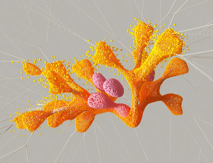
Visualize and Actuate: Plotting Cluster Distributions for Structural Families
The ultimate goal of dimensionality reduction is to actuate biological insights through effective visualization. Once we transform high-dimensional embeddings into a low-dimensional UMAP projection, the next crucial step involves plotting these points and identifying meaningful clusters, often corresponding to structural or functional protein families. We employ powerful visualization libraries like Matplotlib and Seaborn to generate compelling scatter plots of the UMAP output.
For cluster detection, we deploy robust algorithms. HDBSCAN (Hierarchical Density-Based Spatial Clustering of Applications with Noise) stands out for its ability to identify clusters of varying densities and effectively handle noise, making it highly suitable for the often irregular shapes observed in UMAP projections of biological data. Alternatively, K-Means or DBSCAN offer viable options depending on the expected cluster characteristics. After assigning a cluster label to each protein, we color-code the UMAP plot accordingly, instantly revealing the distribution of similar structural families. Furthermore, integrating external metadata, such as known protein family annotations, enzyme classes, or organism origin, enriches these visualizations. We can color points based on these properties, validating existing classifications or uncovering previously unrecognized relationships. This iterative process of UMAP parameter tuning, clustering, and visualization empowers us to decode complex biological systems, transforming raw data into a narrative of molecular discovery and identifying specific leverage points for further experimental investigation.
import matplotlib.pyplot as plt
import seaborn as sns
import pandas as pd
from sklearn.cluster import HDBSCAN # Or KMeans, DBSCAN

def plot_umap_clusters(low_dim_data, labels=None, title="UMAP Projection of Protein Embeddings", metadata_df=None, color_column=None):
    """Visualizes UMAP-reduced embeddings, optionally with cluster labels or metadata."""
    plt.figure(figsize=(12, 10))

    if labels is not None:
        # Option 1: Color by pre-assigned cluster labels
        df = pd.DataFrame(low_dim_data, columns=['UMAP1', 'UMAP2'])
        df['Cluster'] = labels
        sns.scatterplot(x='UMAP1', y='UMAP2', hue='Cluster', data=df, palette='viridis', s=20, alpha=0.7)
    elif metadata_df is not None and color_column is not None and color_column in metadata_df.columns:
        # Option 2: Color by a specific metadata column (e.g., 'protein_family')
        df = pd.DataFrame(low_dim_data, columns=['UMAP1', 'UMAP2'])
        df[color_column] = metadata_df[color_column].values
        # Handle categorical vs. continuous coloring
        if pd.api.types.is_categorical_dtype(df[color_column]) or len(df[color_column].unique()) < 20: # Heuristic for categorical
            sns.scatterplot(x='UMAP1', y='UMAP2', hue=color_column, data=df, palette='tab20', s=20, alpha=0.7)
        else: # Treat as continuous
            sns.scatterplot(x='UMAP1', y='UMAP2', hue=color_column, data=df, cmap='viridis', s=20, alpha=0.7)
    else:
        # Default: Simple scatter plot
        plt.scatter(low_dim_data[:, 0], low_dim_data[:, 1], s=20, alpha=0.7)

    plt.title(title, fontsize=16)
    plt.xlabel('UMAP Dimension 1', fontsize=12)
    plt.ylabel('UMAP Dimension 2', fontsize=12)
    plt.grid(True, linestyle='--', alpha=0.6)
    plt.legend(bbox_to_anchor=(1.05, 1), loc='upper left') # Place legend outside for clarity
    plt.tight_layout()
    plt.show()

def perform_hdbscan_clustering(low_dim_data, min_cluster_size=10, min_samples=None):
    """Applies HDBSCAN for robust density-based clustering."""
    clusterer = HDBSCAN(min_cluster_size=min_cluster_size, min_samples=min_samples)
    cluster_labels = clusterer.fit_predict(low_dim_data)
    return cluster_labels

# Example Usage:
# Assuming 'low_dim_data' is from apply_umap()
# 1. Perform clustering (e.g., HDBSCAN for density-based grouping)
# cluster_labels = perform_hdbscan_clustering(low_dim_data, min_cluster_size=15)

# 2. Visualize with clusters
# plot_umap_clusters(low_dim_data, labels=cluster_labels, title="UMAP with HDBSCAN Clusters")

# 3. If you have metadata, you can load it as a DataFrame and color by a column
# For example, if you have a CSV with protein IDs and known families:
# metadata_df = pd.DataFrame({"ID": ["P1","P2"], "protein_family": ["Kinase", "Receptor"]})
# plot_umap_clusters(low_dim_data, metadata_df=metadata_df, color_column='protein_family', title="UMAP Colored by Protein Family")
Optimize Interpretations: Advanced Strategies & Navigating Pitfalls
Optimizing the interpretation of UMAP projections demands an understanding of advanced strategies and an awareness of common pitfalls. The journey from raw embedding to biological insight is not linear; it involves iterative refinement. We strategically integrate external biological metadata directly into our UMAP analysis. For instance, overlaying enzyme commission (EC) numbers or Gene Ontology (GO) terms onto the UMAP plot allows for rapid validation of cluster integrity and provides immediate functional context. This fusion of computational patterns with established biological knowledge transforms raw visualization into actionable scientific hypotheses.
Evaluating the quality of our UMAP projection extends beyond visual inspection. We can employ metrics like the silhouette score or Davies-Bouldin index to quantitatively assess the compactness and separation of identified clusters. While UMAP excels at preserving topological structure, remember that distances in the UMAP plot are not always directly proportional to distances in the high-dimensional space; focus on connectivity and relative proximity rather than absolute Euclidean distances. Common errors include misinterpreting dense regions as singular clusters without statistical validation, or selecting UMAP parameters that over-emphasize either local noise or overly smooth global structures, thereby obscuring true biological variation. We mitigate these risks through cross-validation, hyperparameter grid search, and expert biological review. Mastering these nuances activates a deeper, more rigorous interpretation, ensuring our computational insights robustly guide experimental design and accelerate discovery.
Key Takeaways
Mastering UMAP for Biological Embeddings
We conquer the challenge of high-dimensional biological embeddings by engineering a precise pipeline to reduce vector dimensions and visualize structural families. This strategic approach transforms complex data into actionable insights for computational bio-engineering.
The Embedding Extraction Pipeline
The core pipeline involves selecting a Protein Language Model (e.g., ProtT5), tokenizing protein sequences, and performing mean pooling on hidden states to generate robust per-sequence embeddings. This foundational step prepares the data for subsequent dimensionality reduction.
UMAP Transformation & Parameter Tuning
UMAP is the critical tool for non-linear dimensionality reduction, preserving local and global data structures. We meticulously tune parameters like n_neighbors (local vs. global balance), min_dist (cluster density), and metric (e.g., 'cosine' for semantic similarity) to optimize the low-dimensional projection.
Visualization and Interpretation
We visualize UMAP output using scatter plots, color-coding points by cluster (e.g., from HDBSCAN) or external metadata. This enables us to actuate biological insights, identifying distinct structural or functional protein families and validating hypotheses with established knowledge. Remember: UMAP distances are not absolute; focus on connectivity.
FAQ
-
What is the primary advantage of UMAP over PCA for visualizing biological embeddings?
UMAP's primary advantage lies in its ability to preserve both local and global data structures within a non-linear manifold. PCA, a linear method, excels at identifying orthogonal directions of maximal variance but often struggles to capture the intricate, non-linear relationships inherent in complex biological data like protein embeddings. UMAP provides a more faithful, topologically accurate low-dimensional representation, revealing nuanced clusters and relationships that PCA might miss or distort.
-
How do we select optimal UMAP parameters (n_neighbors, min_dist) for protein data?
Selecting optimal UMAP parameters is an iterative process demanding biological intuition and systematic exploration. We initiate with default values and then vary
n_neighborsto balance local (smaller values, 5-30) versus global (larger values, 50-200) structure preservation. Simultaneously, we adjustmin_dist(0.0 to 0.5) to control cluster compactness and point separation. We look for projections that create well-separated, biologically coherent clusters, often validating with known structural or functional annotations. There is no single 'optimal' setting; the best parameters emerge through systematic testing and expert interpretation. -
Can UMAP reveal novel protein families or functions?
Absolutely. UMAP empowers us to reveal novel protein families and potentially infer new functions. By visualizing high-dimensional embeddings, UMAP can group together proteins with shared underlying biophysical or evolutionary properties that may not be evident through sequence identity alone. Distinct, well-separated clusters in the UMAP projection, particularly those without prior annotation, strongly indicate novel structural or functional families. This becomes a critical leverage point for hypothesis generation, guiding targeted experimental validation and accelerating the discovery of uncharacterized proteins or functions.