
> Computational Bio-Engineering & Molecular Coding > protein language models and transformers > Decode Protein Transformers: Extract Per-Residue Embeddings
Decode Protein Transformers: Extract Per-Residue Embeddings
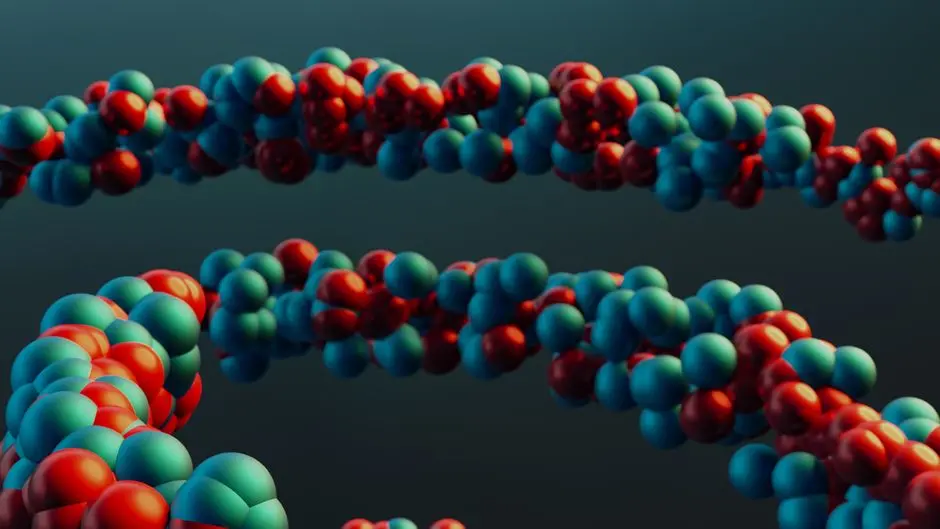
The era of static, one-dimensional protein understanding concludes. We forge a new path, activating the profound insights hidden within advanced computational models. Unlocking per-residue embeddings from protein transformers represents a pivotal leap, offering granular visibility into the intricate dance of amino acids that dictates protein function, interaction, and evolutionary trajectory. This capability is not merely an academic pursuit; it is the strategic leverage point for breakthroughs in drug discovery, precision enzyme engineering, and the deciphering of complex biological mechanisms.
This article guides you through the precise mechanisms and practical implementations to access these dense numerical matrices, capturing the contextual essence of every individual amino acid. We empower you to transition from bulk protein analysis to a nuanced, residue-specific understanding. Prepare to dive deep into the architecture of the advanced architecture of protein language models and transformers, master the code, and unlock a new dimension of biological exploration. This is your blueprint for transforming raw protein sequences into a rich, actionable data landscape.
The Core Mandate: Why Per-Residue Embeddings Drive Discovery
We initiate our journey by establishing the fundamental value proposition of per-residue embeddings. Imagine a protein not as a monolithic entity, but as a dynamic ensemble where each amino acid contributes uniquely to its overall behavior. Traditional protein-level embeddings capture a holistic representation, summarizing the entire sequence into a single vector. While valuable for broad classification or comparison, this approach obscures the fine-grained, localized information crucial for understanding specific biological events. Per-residue embeddings dismantle this limitation, furnishing a distinct numerical vector for every individual amino acid within a protein sequence.
These high-dimensional vectors encapsulate rich contextual information: an amino acid's identity, its position, its immediate chemical environment, and its long-range interactions, all learned from vast corpora of protein sequences. They are not merely positional encodings; they are sophisticated representations reflecting the biochemical role and structural implications of each residue within its specific protein context. This granular insight becomes an indispensable asset. We decode mutation effects with unprecedented precision, pinpointing how a single amino acid alteration propagates through the protein. We delineate active sites, binding interfaces, and functional domains, transforming abstract concepts into quantifiable data. This foundational shift from macroscopic to microscopic understanding propels our ability to engineer novel proteins, design targeted therapeutics, and unravel the molecular basis of disease.
Navigating Transformer Architectures: Pinpointing Hidden States
To successfully extract per-residue embeddings, we must first master the architectural nuances of protein transformer models. These models, often based on the encoder-decoder or encoder-only Transformer architecture, process sequences of amino acids by converting them into numerical tokens, then passing these through multiple layers of self-attention and feed-forward networks. Each encoder block refines the contextual representation of every token. The 'hidden states' are the dense numerical outputs generated by each of these internal layers for every input token.
A critical distinction emerges: which hidden state should we leverage? Early layers typically capture local, syntactic information – akin to basic amino acid physicochemical properties or short-range interactions. As data flows through deeper layers, the representations evolve to incorporate increasingly global, semantic, and functional information, reflecting complex long-range dependencies and higher-order structural motifs. We often target the hidden states of the penultimate or final encoder layer, as these have undergone the most extensive contextualization and integrate information from the entire protein sequence. However, specific tasks might benefit from different layers; experimenting with layers is a key optimization strategy.
When we instantiate a transformer model from libraries like Hugging Face, we configure it to explicitly output these hidden states. The output will typically be a tuple or list of tensors, where each tensor corresponds to the output of a specific layer. Each tensor possesses dimensions representing the batch size, sequence length (including special tokens like [CLS] and [SEP]), and the embedding dimension. Our task is to precisely isolate the tensors corresponding to the amino acid residues, discarding the special tokens which serve as architectural markers rather than biological representations.
import torch
from transformers import AutoTokenizer, AutoModelForMaskedLM

# Define the model identifier for a pre-trained protein transformer like ESM-2
model_name = "facebook/esm2_t6_8M_UR50D" # Example for a smaller ESM-2 model

# Activate the tokenizer and model
tokenizer = AutoTokenizer.from_pretrained(model_name)
model = AutoModelForMaskedLM.from_pretrained(model_name)

# Configure the model to output hidden states
# We must set output_hidden_states=True when calling the model during inference.
# Example for a dummy sequence to check outputs
sequence = "A R N D C Q E G H I L K M F P S T W Y V"
encoded_input = tokenizer(sequence, return_tensors="pt")

# Perform a forward pass, ensuring hidden states are captured
with torch.no_grad():
    outputs = model(**encoded_input, output_hidden_states=True)

# Accessing hidden states: A tuple of tensors, one for each layer's output
# The first element is the input embedding itself.
# The last element typically represents the final layer's hidden states.
hidden_states = outputs.hidden_states

print(f"Number of hidden states (layers + input embedding): {len(hidden_states)}")
print(f"Shape of the final layer's hidden state (batch_size, sequence_length, embedding_dim): {hidden_states[-1].shape}")

# The sequence length includes special tokens [CLS] and [SEP]
# For per-residue embeddings, we usually discard these special tokens.
# For a sequence 'ARND', tokenized might be '[CLS] A R N D [SEP]'
# The actual residue embeddings are at indices 1 to len(sequence).
# For example, to get per-residue embeddings for 'ARND':
# residue_embeddings = hidden_states[-1][:, 1:-1, :]
# print(f"Shape of per-residue embeddings: {residue_embeddings.shape}")
Practical Extraction: Implementing Per-Residue Embedding Capture
We now transition from theoretical understanding to concrete implementation. Extracting per-residue embeddings from protein transformers primarily involves three logical steps: preparing input sequences, executing a forward pass through the model, and precisely capturing the desired hidden states. We leverage established libraries like Hugging Face Transformers, which provide seamless access to state-of-the-art models such as ESM-2.
First, input preparation mandates tokenization. Each protein sequence must be converted into a numerical representation that the model comprehends. The model's tokenizer handles this, adding special tokens (e.g., [CLS] at the start, [SEP] at the end for ESM models) and padding sequences to a uniform length within a batch, crucial for efficient GPU processing. We engineer batches of sequences to optimize computational throughput, especially critical for long proteins or large datasets. Second, we perform a forward pass. Instantiate the pre-trained model (e.g., using AutoModel.from_pretrained) and ensure it is in evaluation mode (model.eval()) to disable dropout and other training-specific behaviors, guaranteeing deterministic outputs. Crucially, we pass output_hidden_states=True to the model's forward method to ensure these internal representations are stored.
Third, we extract and refine the hidden states. The model's output object contains a hidden_states attribute, typically a tuple of tensors. We select the tensor corresponding to the final (or desired intermediate) encoder layer. Each tensor holds embeddings for all tokens in the sequence, including the special [CLS] and [SEP] tokens. A surgical slice operation (e.g., [1:original_seq_len + 1, :]) removes these extraneous tokens, isolating the clean per-residue embeddings. We then transfer these tensors to CPU and convert them to NumPy arrays for subsequent analysis, establishing a robust pipeline for data acquisition.
import torch
from transformers import AutoTokenizer, AutoModel

# Define the model identifier for a pre-trained protein transformer like ESM-2
# Choose an appropriate model size based on your computational resources and task.
# Examples:
# "facebook/esm2_t6_8M_UR50D" (small, fast)
# "facebook/esm2_t30_150M_UR50D" (medium)
# "facebook/esm2_t33_650M_UR50D" (large, high performance, requires more VRAM)
model_name = "facebook/esm2_t30_150M_UR50D"

# Activate the tokenizer and model for feature extraction
# AutoModel is suitable for obtaining embeddings (features), not masked language modeling.
tokenizer = AutoTokenizer.from_pretrained(model_name)
model = AutoModel.from_pretrained(model_name)

# Ensure the model is in evaluation mode for consistent behavior and no dropout
model.eval()

# Move model to GPU if available for accelerated processing
if torch.cuda.is_available():
    model = model.cuda()
    print("Model moved to GPU.")
else:
    print("GPU not available, running on CPU.")

# Prepare your protein sequences (example list)
protein_sequences = [
    "MTYKLILGTLKASLPTGLK",
    "KLRRKRHRRKHNRKRGYRSGYR",
    "MVLSEGEWQLVLHVWAKVEADVAGHGQDLGEALERMFTYFPETTKKGKLFAV"
]

# Process sequences in batches to optimize GPU utilization
batch_size = 2 # Adjust based on your GPU memory
all_per_residue_embeddings = []

for i in range(0, len(protein_sequences), batch_size):
    batch_sequences = protein_sequences[i:i+batch_size]

    # Tokenize the batch of sequences
    # Add_special_tokens=True is default and adds [CLS], [SEP] for ESM.
    # Padding='longest' ensures all sequences in a batch have the same length.
    # Return_tensors='pt' returns PyTorch tensors.
    encoded_input = tokenizer(batch_sequences,
                              return_tensors="pt",
                              padding='longest',
                              truncation=True)

    # Move inputs to GPU if the model is on GPU
    if torch.cuda.is_available():
        encoded_input = {k: v.cuda() for k, v in encoded_input.items()}

    # Perform a forward pass without gradient computation
    with torch.no_grad():
        outputs = model(**encoded_input, output_hidden_states=True)

    # Extract hidden states from the last layer (typically the most contextualized)
    # hidden_states is a tuple where each element is a tensor of shape (batch_size, sequence_length, embedding_dim)
    # The last element `outputs.hidden_states[-1]` corresponds to the final encoder layer output.
    batch_hidden_states = outputs.hidden_states[-1]

    # Iterate through the batch to get per-residue embeddings for each sequence
    for seq_idx in range(len(batch_sequences)):
        # Get the original length of the protein sequence without padding
        # This helps to remove padding tokens if padding='longest' was used.
        original_seq_len = len(batch_sequences[seq_idx])

        # Extract embeddings for actual residues by slicing:
        # [CLS] token is at index 0, [SEP] token is at original_seq_len + 1.
        # So actual residues are from index 1 to original_seq_len (inclusive).
        per_residue_embedding = batch_hidden_states[seq_idx, 1:original_seq_len + 1, :]
        all_per_residue_embeddings.append(per_residue_embedding.cpu().numpy()) # Move to CPU and convert to NumPy

# Print shapes of extracted embeddings
for i, embeddings in enumerate(all_per_residue_embeddings):
    print(f"Sequence {i+1}: '{protein_sequences[i]}' -> Per-residue embedding shape: {embeddings.shape}")

# You now have a list of NumPy arrays, where each array is (num_residues, embedding_dim)
# These embeddings are ready for downstream analysis.
Post-Processing and Interpretation: Maximizing Embeddings' Actionable Value
Extracting embeddings is merely the first conquest; deriving actionable intelligence mandates sophisticated post-processing and astute interpretation. We must transform raw numerical matrices into interpretable biological insights. The high dimensionality of per-residue embeddings (e.g., 320 or 1280 dimensions for ESM-2 models) necessitates dimensionality reduction techniques for visualization and certain analytical tasks. Algorithms like UMAP (Uniform Manifold Approximation and Projection) and t-SNE (t-distributed Stochastic Neighbor Embedding) excel at projecting these complex data points into two or three dimensions, preserving intricate local and global relationships. This enables us to visualize clusters of functionally similar residues or identify outlier residues with unique contexts.
Mapping these reduced dimensions back to their original residue positions within the protein sequence is paramount. We color-code residues based on their cluster assignment or projection values, revealing hidden patterns on the protein structure. For downstream applications, these embeddings become powerful features. We train machine learning models to predict post-translational modifications, ligand binding sites, stability effects of mutations, or specific functional domains. The embeddings effectively act as a universal language for describing residue context.
Adopting best practices optimizes our analytical rigor. Normalize embeddings before computing distances or applying clustering algorithms to prevent biases from varying vector magnitudes. Carefully select the transformer layer for extraction; the final layer often captures the most integrated information, but intermediate layers might retain specific structural or local physicochemical properties. A common pitfall involves misinterpreting clusters without biological validation; always correlate computational findings with known experimental data. We engineer this comprehensive strategy to transform dense matrices into profound biological discoveries.
import numpy as np
from sklearn.decomposition import PCA
from umap import UMAP
import matplotlib.pyplot as plt
import seaborn as sns

# Assume 'all_per_residue_embeddings' is a list of NumPy arrays
# from the previous code block.
# Example: Convert list of (residues, embedding_dim) to a single (total_residues, embedding_dim) array
# This is often necessary for dimensionality reduction techniques.

# For demonstration, let's create a dummy list of embeddings
# In a real scenario, this would come from the extraction step
dummy_embeddings = [
    np.random.rand(19, 320), # Protein 1 (19 residues, 320 dim for esm2_t30_150M_UR50D)
    np.random.rand(22, 320), # Protein 2
    np.random.rand(34, 320)  # Protein 3
]

# Concatenate all per-residue embeddings into a single matrix for global analysis
combined_embeddings = np.vstack(dummy_embeddings)
print(f"Combined embeddings shape for dimensionality reduction: {combined_embeddings.shape}")

# 1. Dimensionality Reduction (e.g., UMAP or PCA)
# UMAP is excellent for visualizing high-dimensional data, preserving local and global structure.
# PCA is useful for understanding variance and for some simpler tasks.

# UMAP transformation
print("Applying UMAP for dimensionality reduction...")
umap_reducer = UMAP(n_components=2, random_state=42)
reduced_embeddings_umap = umap_reducer.fit_transform(combined_embeddings)

# PCA transformation (for comparison or alternative view)
print("Applying PCA for dimensionality reduction...")
pca_reducer = PCA(n_components=2, random_state=42)
reduced_embeddings_pca = pca_reducer.fit_transform(combined_embeddings)

print(f"UMAP reduced embeddings shape: {reduced_embeddings_umap.shape}")
print(f"PCA reduced embeddings shape: {reduced_embeddings_pca.shape}")

# 2. Visualization (Example for UMAP)
plt.figure(figsize=(10, 8))
sns.scatterplot(x=reduced_embeddings_umap[:, 0], y=reduced_embeddings_umap[:, 1],
                hue=np.repeat(np.arange(len(dummy_embeddings)), [len(e) for e in dummy_embeddings]),
                palette='viridis', s=20, alpha=0.7)
plt.title('UMAP Projection of Per-Residue Embeddings')
plt.xlabel('UMAP Dimension 1')
plt.ylabel('UMAP Dimension 2')
plt.colorbar(label='Protein Index')
plt.show()

# 3. Downstream Task Example: Preparing for Clustering
# We can apply clustering algorithms (e.g., KMeans, DBSCAN) to the reduced or original embeddings.
from sklearn.cluster import KMeans

print("Applying KMeans clustering on UMAP-reduced embeddings...")
kmeans = KMeans(n_clusters=3, random_state=42, n_init=10) # Example: 3 clusters
clusters = kmeans.fit_predict(reduced_embeddings_umap)

plt.figure(figsize=(10, 8))
sns.scatterplot(x=reduced_embeddings_umap[:, 0], y=reduced_embeddings_umap[:, 1],
                hue=clusters, palette='deep', s=20, alpha=0.8)
plt.title('UMAP Projection with KMeans Clusters')
plt.xlabel('UMAP Dimension 1')
plt.ylabel('UMAP Dimension 2')
plt.colorbar(label='Cluster')
plt.show()

# Best Practice: Normalization
# Before certain analyses (e.g., clustering, calculating distances), normalization can be beneficial.
normalized_embeddings = combined_embeddings / np.linalg.norm(combined_embeddings, axis=1, keepdims=True)
print(f"Shape of normalized embeddings: {normalized_embeddings.shape}")
Key Takeaways
Unlocking Granular Protein Insights with Per-Residue Embeddings
We establish per-residue embeddings as critical tools for deep, granular understanding of protein function. Unlike holistic protein embeddings, these vectors capture the unique contextual role of each amino acid, facilitating precise analysis of mutation effects, active sites, and functional domains. This empowers breakthroughs in drug discovery and protein engineering.
Strategic Navigation of Transformer Hidden States
We mandate understanding protein transformer architecture, particularly encoder layers and hidden states. Each layer refines contextual information, with deeper layers capturing global semantic data. We target penultimate or final layer hidden states for comprehensive contextualization, ensuring explicit configuration for outputting these states during model inference.
Precision Implementation for Embedding Extraction
We detail a three-step implementation: input tokenization, forward pass, and precise hidden state capture. Leveraging Hugging Face Transformers, we batch process sequences, pass output_hidden_states=True, and surgically slice output tensors to isolate per-residue embeddings, discarding special tokens and padding. This pipeline prepares embeddings for downstream analysis.
Transforming Embeddings into Actionable Biological Intelligence
We post-process embeddings using dimensionality reduction (UMAP, t-SNE) for visualization and pattern discovery, mapping insights back to protein structures. These embeddings become powerful features for machine learning, predicting diverse biological properties. We enforce best practices like normalization and careful layer selection, validating findings with experimental data to convert numerical matrices into profound biological discoveries.
FAQ
-
What distinguishes per-residue embeddings from whole-protein embeddings?
Per-residue embeddings forge a distinct numerical vector for every individual amino acid within a protein, capturing its unique contextual information (local environment, long-range interactions). Whole-protein embeddings, conversely, condense the entire protein sequence into a single vector, representing its holistic features. We utilize per-residue embeddings for granular analyses like mutation effect prediction or active site identification, while whole-protein embeddings serve broader classification or comparative tasks.
-
Which transformer layer should I extract embeddings from?
We typically target the hidden states of the penultimate or final encoder layer. These layers integrate the most extensive contextual information from the entire protein sequence. However, early layers capture more local, physicochemical properties. The optimal layer depends on your specific biological task; we advocate for experimentation across layers to determine which best correlates with your target property or phenomenon.
-
How do I handle proteins with varying sequence lengths during embedding extraction?
When processing protein sequences in batches, transformer tokenizers (like those in Hugging Face) automatically handle variable lengths through padding. They add special 'padding' tokens to shorter sequences to match the longest sequence in the batch. We ensure that after extracting the hidden states, we surgically slice these tensors to remove the embeddings corresponding to these padding tokens and the special [CLS]/[SEP] tokens, retrieving only the embeddings for the actual amino acid residues.