
> Bio-engineering & bioinformatics pipelines > Vector Search and Similarity Systems > Benchmark Distances: Protein Embeddings & Molecular Similarity Metrics
Benchmark Distances: Protein Embeddings & Molecular Similarity Metrics
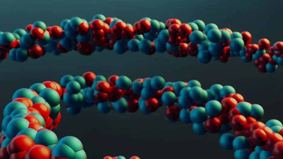
Activate the full potential of your bioinformatics pipelines by mastering molecular similarity. Protein embeddings, numerical representations of complex biological structures, fuel breakthroughs in drug discovery, functional annotation, and evolutionary analysis. Yet, the true power of these embeddings emerges only when coupled with the correct distance metric. This resource dissects the critical distinctions between Cosine, Euclidean, and Manhattan metrics, illuminating their unique strengths and weaknesses for evaluating protein similarity. We engineer a practical framework, demonstrating each metric's application with Python, empowering you to make informed decisions that dictate the precision and relevance of your biological insights. Understanding these metrics is paramount to effectively implement large-scale vector search for molecular and protein embeddings, ensuring your similarity systems deliver optimal biological relevance. Forge ahead to unlock hidden relationships and accelerate discovery within the vast landscape of biological data.
Architecting Protein Embeddings and Similarity Foundations
We commence our exploration by solidifying the foundational concepts of protein embeddings and molecular similarity. Protein embeddings are dense, high-dimensional numerical vectors generated by advanced machine learning models, such as transformers or recurrent neural networks, trained on vast protein sequence or structure datasets. These vectors encapsulate intricate biophysical, biochemical, and evolutionary features of proteins, translating complex biological information into a computationally tractable format. This numerical representation empowers us to perform quantitative comparisons that transcend traditional sequence alignment limitations, capturing nuanced relationships. Imagine each protein as a point in a multi-dimensional space; the closer two points are, the more similar their underlying biological properties.
The imperative for molecular similarity arises across critical biological frontiers: identifying novel drug targets, predicting protein function from sequence, engineering proteins with enhanced properties, and deciphering evolutionary pathways. Activating robust similarity metrics is not merely an analytical step; it is a strategic decision that directly impacts the biological relevance and actionable insights derived from your data. Without a judicious choice of metric, our powerful embeddings remain underutilized, potentially leading to misinterpretations or missed opportunities. We forge the pathway to optimal metric selection by first establishing a common ground for protein representation.
# Python setup for generating dummy protein embeddings
import numpy as np

# Set a seed for reproducibility
np.random.seed(42)

# Define the number of proteins and embedding dimension
num_proteins = 100
embedding_dim = 128 # A common dimension for protein embeddings

# Generate dummy protein embeddings (e.g., from a deep learning model)
# These are typically floats, often normalized, representing complex features.
protein_embeddings = np.random.rand(num_proteins, embedding_dim)

# Display the shape of the generated embeddings
print(f"Shape of protein_embeddings: {protein_embeddings.shape}")

# Example of selecting two proteins for similarity comparison
protein_A_embedding = protein_embeddings[0]
protein_B_embedding = protein_embeddings[1]
protein_C_embedding = protein_embeddings[2] # A third protein for comparison

print(f"Embedding for Protein A (first 5 values): {protein_A_embedding[:5]}")
print(f"Embedding for Protein B (first 5 values): {protein_B_embedding[:5]}")
print(f"Embedding for Protein C (first 5 values): {protein_C_embedding[:5]}")
Decrypting Cosine Similarity for Directional Insight
We decode Cosine Similarity as a paramount metric for capturing directional relationships between protein embeddings. This metric evaluates the cosine of the angle between two vectors, ranging from -1 (perfectly opposite) to 1 (perfectly aligned), with 0 indicating orthogonality. Crucially, Cosine Similarity focuses solely on the orientation of the vectors in space, rendering it insensitive to their magnitudes. This characteristic makes it exceptionally potent when the absolute 'length' or magnitude of an embedding might not correlate directly with biological significance, or when embeddings are not inherently magnitude-normalized. For instance, if a larger embedding magnitude simply reflects more amino acids without implying greater functional 'strength', Cosine Similarity bypasses this potential noise.
Deploy Cosine Similarity when your primary objective is to identify proteins with similar functional roles, shared binding motifs, or comparable structural folds, where the 'direction' of features in the embedding space is indicative of biological homology. It excels in scenarios where sparse data might otherwise distort distance calculations based on absolute values. However, understand its inherent limitation: by ignoring magnitude, it might overlook instances where the 'strength' or 'intensity' of certain features, reflected in vector length, carries biological meaning. For example, if a stronger signal in an embedding indicates a more active site, Cosine Similarity would not differentiate between a weak and strong signal, provided their directions are identical. This surgical understanding guides its optimal application.
# Python implementation of Cosine Similarity
import numpy as np
from scipy.spatial.distance import cosine

# Assume protein_A_embedding and protein_B_embedding are defined from previous step
# For this example, let's redefine them for clarity if running independently
np.random.seed(42)
embedding_dim = 128
protein_A_embedding = np.random.rand(embedding_dim)
protein_B_embedding = np.random.rand(embedding_dim)
protein_C_embedding = np.random.rand(embedding_dim)

# --- Manual Calculation of Cosine Similarity ---
# Cosine similarity measures the cosine of the angle between two non-zero vectors.
# A value of 1 means identical direction, 0 means orthogonal, -1 means opposite direction.
# Formula: (A . B) / (||A|| * ||B||)

def calculate_cosine_similarity(vec1, vec2):
    dot_product = np.dot(vec1, vec2)
    norm_vec1 = np.linalg.norm(vec1)
    norm_vec2 = np.linalg.norm(vec2)
    if norm_vec1 == 0 or norm_vec2 == 0:
        return 0.0 # Handle zero vectors gracefully
    return dot_product / (norm_vec1 * norm_vec2)

cosine_sim_AB_manual = calculate_cosine_similarity(protein_A_embedding, protein_B_embedding)
cosine_sim_AC_manual = calculate_cosine_similarity(protein_A_embedding, protein_C_embedding)
print(f"Manual Cosine Similarity (A, B): {cosine_sim_AB_manual:.4f}")
print(f"Manual Cosine Similarity (A, C): {cosine_sim_AC_manual:.4f}")

# --- Using SciPy's Cosine Distance (1 - similarity) ---
# SciPy's 'cosine' function calculates cosine distance, not similarity.
# Cosine Distance = 1 - Cosine Similarity

cosine_dist_AB_scipy = cosine(protein_A_embedding, protein_B_embedding)
cosine_sim_AB_scipy = 1 - cosine_dist_AB_scipy

cosine_dist_AC_scipy = cosine(protein_A_embedding, protein_C_embedding)
cosine_sim_AC_scipy = 1 - cosine_dist_AC_scipy

print(f"SciPy Cosine Similarity (A, B): {cosine_sim_AB_scipy:.4f}")
print(f"SciPy Cosine Similarity (A, C): {cosine_sim_AC_scipy:.4f}")

# Example: If vectors are identical, similarity should be 1
cosine_sim_AA = calculate_cosine_similarity(protein_A_embedding, protein_A_embedding)
print(f"Cosine Similarity (A, A): {cosine_sim_AA:.4f}")
Navigating Euclidean Distance for Magnitude-Sensitive Proximity
We navigate Euclidean Distance as the quintessential measure of straight-line proximity in the embedding space. Also known as L2 norm, Euclidean Distance calculates the square root of the sum of squared differences between corresponding elements of two vectors. This metric is profoundly sensitive to the absolute magnitudes of the embedding dimensions. A larger difference in any single dimension contributes quadratically to the overall distance, making it effective for distinguishing proteins where subtle shifts in feature intensity or absolute values carry significant biological weight. Consider a scenario where an embedding dimension encodes the concentration of a specific amino acid or the magnitude of a binding affinity; Euclidean Distance will directly capture and emphasize these quantitative variations.
Deploy Euclidean Distance when the absolute dissimilarity across all features is critical, such as in analyses of conformational changes, quantitative structural variations, or scenarios where the overall 'amount' or 'strength' of specific molecular properties defines biological divergence. It shines when working with dense embeddings where all dimensions contribute meaningfully to the biological interpretation. However, we must activate a critical awareness of its vulnerabilities: Euclidean Distance is highly susceptible to the 'curse of dimensionality' in very high-dimensional spaces, where all points tend to become equidistant. Furthermore, unscaled features or features with disparate ranges can disproportionately influence the distance, necessitating rigorous preprocessing like normalization or standardization of embeddings to ensure fair comparison and prevent dominant features from overshadowing others. Overlook this, and your similarity landscape becomes distorted.
# Python implementation of Euclidean Distance
import numpy as np
from scipy.spatial.distance import euclidean

# Assume protein_A_embedding, protein_B_embedding, protein_C_embedding are defined
# For this example, let's redefine them for clarity if running independently
np.random.seed(42)
embedding_dim = 128
protein_A_embedding = np.random.rand(embedding_dim)
protein_B_embedding = np.random.rand(embedding_dim)
protein_C_embedding = np.random.rand(embedding_dim)

# --- Manual Calculation of Euclidean Distance ---
# Euclidean distance measures the straight-line distance between two points in Euclidean space.
# Formula: sqrt(sum((p_i - q_i)^2))

def calculate_euclidean_distance(vec1, vec2):
    return np.linalg.norm(vec1 - vec2)

euclidean_dist_AB_manual = calculate_euclidean_distance(protein_A_embedding, protein_B_embedding)
euclidean_dist_AC_manual = calculate_euclidean_distance(protein_A_embedding, protein_C_embedding)
print(f"Manual Euclidean Distance (A, B): {euclidean_dist_AB_manual:.4f}")
print(f"Manual Euclidean Distance (A, C): {euclidean_dist_AC_manual:.4f}")

# --- Using SciPy's Euclidean Distance ---

euclidean_dist_AB_scipy = euclidean(protein_A_embedding, protein_B_embedding)
euclidean_dist_AC_scipy = euclidean(protein_A_embedding, protein_C_embedding)

print(f"SciPy Euclidean Distance (A, B): {euclidean_dist_AB_scipy:.4f}")
print(f"SciPy Euclidean Distance (A, C): {euclidean_dist_AC_scipy:.4f}")

# Example: If vectors are identical, distance should be 0
euclidean_dist_AA = calculate_euclidean_distance(protein_A_embedding, protein_A_embedding)
print(f"Euclidean Distance (A, A): {euclidean_dist_AA:.4f}")

# Demonstrate normalization impact (important for Euclidean)
protein_A_scaled = protein_A_embedding * 10 # Scale one vector
euclidean_dist_A_A_scaled = calculate_euclidean_distance(protein_A_embedding, protein_A_scaled)
print(f"Euclidean Distance (A, A_scaled): {euclidean_dist_A_A_scaled:.4f}")
# Cosine similarity would be 1 for A and A_scaled, highlighting the difference
print(f"Cosine Similarity (A, A_scaled): {calculate_cosine_similarity(protein_A_embedding, protein_A_scaled):.4f}")

Harnessing Manhattan Distance for Feature-Wise Discrepancy
We harness Manhattan Distance, also known as L1 norm or City Block Distance, to dissect feature-wise discrepancies between protein embeddings. This metric calculates the sum of the absolute differences between the corresponding coordinates of two vectors. Unlike Euclidean, which squares differences, Manhattan Distance sums linear differences. This characteristic renders it less sensitive to outliers or extreme differences in a single dimension, as large deviations do not get quadratically amplified. Imagine navigating a city grid; Manhattan Distance measures the path along the grid lines, emphasizing the individual contributions of each orthogonal movement rather than the direct diagonal. This makes it particularly valuable when each dimension of your protein embedding represents an independent, interpretable feature, and you prioritize understanding the cumulative absolute deviation across these features.
Deploy Manhattan Distance when your objective is to identify protein similarities based on the collective deviation of specific, individual attributes. It excels in scenarios where robustness to sporadic large differences is critical, or when analyzing sparse embeddings where many dimensions might be zero. It provides a more transparent view of the contribution of each dimension to the overall dissimilarity, which can be advantageous for feature selection or interpreting feature importance in biological contexts. For instance, if your embeddings encode counts of specific motifs or domain presence, Manhattan Distance directly quantifies the aggregate count difference. However, recognize its limitation: Manhattan Distance might be less intuitive in very high-dimensional continuous spaces, and its 'grid-like' nature might not optimally capture complex, non-orthogonal relationships inherent in some biological data. We optimize its application by aligning it with the specific granularity of biological inquiry.
# Python implementation of Manhattan Distance
import numpy as np
from scipy.spatial.distance import cityblock # SciPy uses 'cityblock' for Manhattan distance

# Assume protein_A_embedding, protein_B_embedding, protein_C_embedding are defined
# For this example, let's redefine them for clarity if running independently
np.random.seed(42)
embedding_dim = 128
protein_A_embedding = np.random.rand(embedding_dim)
protein_B_embedding = np.random.rand(embedding_dim)
protein_C_embedding = np.random.rand(embedding_dim)

# --- Manual Calculation of Manhattan Distance ---
# Manhattan distance (L1 norm) measures the sum of the absolute differences between the coordinates.
# Formula: sum(|p_i - q_i|)

def calculate_manhattan_distance(vec1, vec2):
    return np.sum(np.abs(vec1 - vec2))

manhattan_dist_AB_manual = calculate_manhattan_distance(protein_A_embedding, protein_B_embedding)
manhattan_dist_AC_manual = calculate_manhattan_distance(protein_A_embedding, protein_C_embedding)
print(f"Manual Manhattan Distance (A, B): {manhattan_dist_AB_manual:.4f}")
print(f"Manual Manhattan Distance (A, C): {manhattan_dist_AC_manual:.4f}")

# --- Using SciPy's Cityblock (Manhattan) Distance ---

manhattan_dist_AB_scipy = cityblock(protein_A_embedding, protein_B_embedding)
manhattan_dist_AC_scipy = cityblock(protein_A_embedding, protein_C_embedding)

print(f"SciPy Manhattan Distance (A, B): {manhattan_dist_AB_scipy:.4f}")
print(f"SciPy Manhattan Distance (A, C): {manhattan_dist_AC_scipy:.4f}")

# Example: If vectors are identical, distance should be 0
manhattan_dist_AA = calculate_manhattan_distance(protein_A_embedding, protein_A_embedding)
print(f"Manhattan Distance (A, A): {manhattan_dist_AA:.4f}")

# Demonstrate robustness to outliers compared to Euclidean
# Create two vectors, one with a large outlier feature
vec1 = np.array([1, 2, 3, 100])
vec2 = np.array([1, 2, 3, 4])

euclidean_outlier_impact = euclidean(vec1, vec2)
manhattan_outlier_impact = cityblock(vec1, vec2)

print(f"Euclidean with outlier: {euclidean_outlier_impact:.4f}") # Large impact
print(f"Manhattan with outlier: {manhattan_outlier_impact:.4f}") # Less quadratic impact

Optimizing Metric Selection: Best Practices and Pitfalls
We conclude our deep dive by synthesizing best practices for optimizing metric selection, transforming complexity into actionable strategy. There exists no universal 'best' distance metric; the optimal choice is surgically dependent on the specific biological question, the nature of the protein embeddings, and the inherent properties of your dataset. A critical insider tip: always interrogate the underlying biological meaning encoded by your embeddings. Do higher magnitude values signify greater importance, or are they mere artifacts of the embedding process? This understanding dictates whether magnitude-sensitive metrics like Euclidean or Manhattan are appropriate, or if Cosine Similarity, which focuses purely on direction, is superior.
A common pitfall involves neglecting preprocessing. Before deploying Euclidean or Manhattan distances, we vigorously recommend normalizing or standardizing your embeddings. L2 normalization (scaling vectors to unit length) makes Euclidean distance behave more akin to Cosine Similarity, effectively focusing on direction while still considering magnitude differences in a controlled manner. Feature scaling (e.g., using StandardScaler) ensures that no single dimension with a larger numerical range disproportionately biases the distance calculation. Another crucial consideration is the density of your embeddings. For sparse representations, where many dimensions are zero, Cosine and Manhattan can often outperform Euclidean. We also activate iterative validation: experiment with different metrics, evaluate their performance against ground truth biological relationships, and refine your choice. The decisive engineer validates, never assumes. This iterative approach ensures that your chosen metric genuinely decodes biological reality, not just numerical proximity.
# Python example demonstrating how embedding normalization impacts Euclidean and Cosine similarity.
import numpy as np
from scipy.spatial.distance import euclidean, cosine

# Set a seed for reproducibility
np.random.seed(42)

# Original embeddings
vec1 = np.array([1, 2, 3, 4]).astype(float)
vec2 = np.array([1.1, 2.2, 3.3, 4.4]).astype(float) # Similar direction, slightly larger magnitude
vec3 = np.array([4, 3, 2, 1]).astype(float)  # Different direction, similar magnitude to vec1

print("--- Original Vectors ---")
print(f"Vec1: {vec1}")
print(f"Vec2: {vec2}")
print(f"Vec3: {vec3}")

print("\n--- Raw Metric Calculations ---")
print(f"Euclidean(vec1, vec2): {euclidean(vec1, vec2):.4f}") # Small Euclidean dist
print(f"Euclidean(vec1, vec3): {euclidean(vec1, vec3):.4f}") # Larger Euclidean dist

print(f"Cosine(vec1, vec2): {1 - cosine(vec1, vec2):.4f}") # High Cosine sim
print(f"Cosine(vec1, vec3): {1 - cosine(vec1, vec3):.4f}") # Lower Cosine sim

# --- L2 Normalization (Unit Vector) ---
# Normalizing embeddings to unit length (L2 norm = 1) is a common preprocessing step,
# especially for Euclidean distance when magnitude is not relevant, or to make Euclidean
# behave more like Cosine similarity.

def normalize_vector(vec):
    norm = np.linalg.norm(vec)
    if norm == 0:
        return vec
    return vec / norm

vec1_norm = normalize_vector(vec1)
vec2_norm = normalize_vector(vec2)
vec3_norm = normalize_vector(vec3)

print("\n--- L2 Normalized Vectors ---")
print(f"Vec1 (normed): {vec1_norm[:3]}... Norm: {np.linalg.norm(vec1_norm):.2f}")
print(f"Vec2 (normed): {vec2_norm[:3]}... Norm: {np.linalg.norm(vec2_norm):.2f}")
print(f"Vec3 (normed): {vec3_norm[:3]}... Norm: {np.linalg.norm(vec3_norm):.2f}")

print("\n--- Metrics after L2 Normalization ---")
# For L2 normalized vectors, Euclidean distance is directly related to Cosine similarity
# Euclidean Distance^2 = 2 * (1 - Cosine Similarity)
print(f"Euclidean(vec1_norm, vec2_norm): {euclidean(vec1_norm, vec2_norm):.4f}")
print(f"Euclidean(vec1_norm, vec3_norm): {euclidean(vec1_norm, vec3_norm):.4f}")

print(f"Cosine(vec1_norm, vec2_norm): {1 - cosine(vec1_norm, vec2_norm):.4f}")
print(f"Cosine(vec1_norm, vec3_norm): {1 - cosine(vec1_norm, vec3_norm):.4f}")

# Key takeaway: Normalizing changes the behavior of Euclidean distance. If embeddings are L2 normalized,
# Euclidean distance and Cosine similarity become directly related, effectively measuring the same underlying angle.

# --- Insider Tip: Feature Scaling for Manhattan/Euclidean ---
# If embedding dimensions represent different biological units or scales,
# consider StandardScaler or MinMaxScaler from sklearn.preprocessing for individual features.
# Example (conceptual, as we don't have explicit feature meanings here):
# from sklearn.preprocessing import StandardScaler
# scaler = StandardScaler()
# scaled_embeddings = scaler.fit_transform(protein_embeddings)
# Then calculate metrics on scaled_embeddings.
Key Takeaways
Protein Embeddings: Core Concept
Protein embeddings transform complex biological information (sequences/structures) into fixed-size numerical vectors. These vectors capture biophysical, biochemical, and evolutionary features, enabling quantitative similarity comparisons for drug discovery, function prediction, and evolutionary analysis. Choosing the correct distance metric is paramount for relevant biological insights.
Cosine Similarity: Directional Insight
Mechanism: Measures the cosine of the angle between two vectors (range -1 to 1). Insensitive to vector magnitude, focuses on direction.
Strengths: Excellent for functional similarity, shared motifs, structural folds where relative direction matters. Robust to magnitude variations and sparse data.
Limitations: Ignores magnitude, potentially missing biological significance linked to feature 'strength'.
Use Case: Identifying functionally homologous proteins.
Euclidean Distance: Magnitude-Sensitive Proximity
Mechanism: Measures straight-line distance (L2 norm) between two points. Highly sensitive to absolute differences and magnitudes.
Strengths: Ideal for quantitative structural changes, absolute property differences. Captures overall 'amount' or 'strength' of molecular features.
Limitations: Highly susceptible to 'curse of dimensionality.' Requires rigorous preprocessing (normalization/standardization) to prevent disproportionate feature influence.
Use Case: Quantifying global conformational changes.
Manhattan Distance: Feature-Wise Discrepancy
Mechanism: Sum of absolute differences (L1 norm) between coordinates. Less sensitive to outliers than Euclidean.
Strengths: Robust to extreme differences in single dimensions. Provides clear insight into cumulative individual feature contributions. Good for sparse data.
Limitations: Less intuitive in very high-dimensional continuous spaces. Might not capture complex, non-orthogonal relationships well.
Use Case: Analyzing aggregate differences across specific interpretable features (e.g., motif counts).
Optimizing Metric Selection: Best Practices
No single 'best' metric exists; choice depends on biological question and data. Always interrogate the biological meaning of embedding magnitudes. Preprocess embeddings: L2 normalization for Euclidean (to focus on direction) or feature scaling for disparate ranges. Validate chosen metrics against biological ground truth. Experiment with multiple metrics for a comprehensive view.
FAQ
-
Why are protein embeddings used instead of raw sequences for similarity?
Protein embeddings convert complex, variable-length sequence or structural data into fixed-size, dense numerical vectors. This allows machine learning algorithms to process biological information efficiently, capturing intricate biophysical properties, evolutionary relationships, and functional motifs that are difficult to discern directly from raw sequences. Embeddings represent proteins in a continuous, high-dimensional space where mathematical operations, like distance calculations, are meaningful.
-
When should I prioritize magnitude over direction in protein similarity?
Prioritize magnitude when the absolute 'strength' or 'intensity' of features within your embeddings holds biological significance. For example, if a specific embedding dimension quantifies the presence of a critical binding site or the activity level of an enzyme, then changes in magnitude directly reflect changes in these properties. Euclidean and Manhattan distances are well-suited for these scenarios, as they are sensitive to the absolute differences in feature values.
-
Can I use multiple distance metrics for the same analysis?
Absolutely. Employing multiple distance metrics can provide a more comprehensive understanding of molecular similarity. Different metrics highlight distinct aspects of the embedding space. For example, Cosine Similarity might reveal functional clusters, while Euclidean Distance might separate proteins based on structural changes that alter overall magnitude. Comparing results from various metrics can offer a richer, multi-faceted perspective on your biological data, acting as a powerful validation tool.
-
What is the 'curse of dimensionality' and how does it affect distance metrics?
The 'curse of dimensionality' refers to phenomena that arise when analyzing data in high-dimensional spaces. In the context of distance metrics, as dimensionality increases, all data points tend to become nearly equidistant from each other, making it challenging to distinguish meaningful similarities or dissimilarities. Euclidean Distance is particularly susceptible to this, as differences across many dimensions can dilute true proximity. Cosine Similarity is generally more robust to this effect because it focuses on angular separation rather than absolute distance.
-
Is normalization always necessary before calculating distance metrics?
Normalization is not always strictly 'necessary' but is almost always a 'best practice,' especially for Euclidean and Manhattan distances. If embedding dimensions have vastly different scales or ranges, or if the magnitude of an embedding is irrelevant to your biological question, then normalization (e.g., L2 normalization) prevents certain features from dominating the distance calculation. For Cosine Similarity, embeddings are often implicitly or explicitly normalized, as its calculation inherently focuses on vector direction.