
> Bio-engineering & bioinformatics pipelines > Vector Search and Similarity Systems > Forge Protein Insights: Cosine Similarity Search in Python
Forge Protein Insights: Cosine Similarity Search in Python
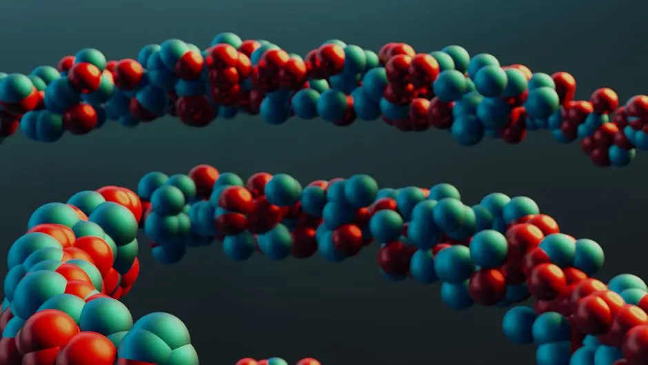
Unlock the profound relationships hidden within protein sequences by mastering vector similarity. Proteins, the workhorses of life, drive countless biological processes. Their functional similarities often correlate with structural resemblances and evolutionary pathways, yet discerning these connections at scale presents a formidable challenge. Leveraging the power of protein embeddings transforms complex sequences into numerical vectors, making their intrinsic properties quantifiable and comparable.
This resource engineers a robust pipeline for computing cosine similarity between protein embeddings using Python, empowering you to identify closely related protein sequences with precision. We activate a strategy that moves beyond simple sequence alignment, diving into a high-dimensional space where functional and evolutionary signals resonate. Expect to decode the core principles, implement practical Python solutions, and optimize for performance, ensuring your biological exploration is both rigorous and scalable. Our objective is to guide you through the process, from generating synthetic embeddings to interpreting the biological significance of similarity scores. This foundational knowledge is crucial for anyone looking to implement large-scale vector search for molecular and protein embeddings, providing a bedrock for advanced bioinformatic applications and accelerating discovery in areas like drug design and protein engineering.
Decode Protein Embeddings: Vectors of Biological Information
Embark on the journey of transforming complex biological sequences into quantifiable vectors. Protein embeddings distill the intricate information of a protein—its sequence, structure, and functional context—into a dense numerical representation, typically a high-dimensional vector. These vectors, often generated by sophisticated deep learning models (e.g., ESM, ProtT5), capture nuanced relationships that traditional sequence alignments might overlook. Each dimension within the vector encodes a learned feature, collectively painting a comprehensive digital portrait of the protein. We embrace this paradigm shift, moving beyond mere character strings to a landscape of meaningful numerical patterns.
The strategic advantage of embeddings lies in their ability to represent biological similarity as geometric proximity in a vector space. Proteins with similar functions, structures, or evolutionary origins will likely possess embedding vectors that point in similar directions. Our mission centers on exploiting this property through cosine similarity. Cosine similarity measures the cosine of the angle between two non-zero vectors, effectively quantifying their directional alignment regardless of their magnitude. A value of 1 signifies identical direction (maximum similarity), -1 indicates opposite direction (maximum dissimilarity), and 0 suggests orthogonality (no relationship). This metric emerges as the gold standard for comparing protein embeddings because it focuses purely on the shared orientation of features, providing a robust and intuitive measure of relatedness that bypasses issues of vector length variation.
Activating this computational lens on biology empowers us to rapidly identify homologous proteins, predict unknown functions, and explore evolutionary relationships with unprecedented efficiency. We bypass the computational intensity of direct sequence comparisons for large datasets, replacing it with a vector-based approach that is both scalable and highly informative. Mastering protein embeddings and their similarity metrics is not merely a technical skill; it is a gateway to accelerating fundamental biological discovery and engineering novel solutions in biomedicine and biotechnology. We leverage Python's robust scientific computing libraries to forge these insights, establishing a clear path from raw data to actionable biological intelligence.
# Python environment setup for protein embedding simulation
import numpy as np
from sklearn.preprocessing import normalize

print("Environment ready for protein embedding simulation.")

# --- Code for Protein Embedding Simulation (Conceptual) ---
# In a real-world scenario, protein embeddings would be generated
# by pre-trained deep learning models (e.g., ESM, ProtT5, AlphaFold's representations).
# Here, we simulate them as high-dimensional NumPy arrays.

def generate_protein_embedding(dimension=768):
    """
    Simulates a protein embedding vector.
    In reality, this comes from a pre-trained model.
    """
    # Embeddings often have values that can be positive or negative.
    # Using random normal distribution to simulate diverse features.
    embedding = np.random.randn(dimension)
    return embedding

# Example: Generate embeddings for a few proteins
protein_ids = ["Protein_A", "Protein_B", "Protein_C", "Protein_D"]
embeddings_dict = {}

for pid in protein_ids:
    embeddings_dict[pid] = generate_protein_embedding(dimension=768)
    print(f"Generated embedding for {pid} with shape {embeddings_dict[pid].shape}")

# It's good practice to normalize embeddings, especially for cosine similarity,
# as it ensures they all lie on the unit sphere, making direction the sole factor.
# While cosine similarity itself normalizes, pre-normalizing can sometimes
# offer marginal performance benefits or align with specific model outputs.

def normalize_embeddings(embeddings_dict):
    normalized_embeddings = {}
    for pid, embedding in embeddings_dict.items():
        # Reshape for sklearn.preprocessing.normalize to handle a single sample
        normalized_embedding = normalize(embedding.reshape(1, -1), axis=1)[0]
        normalized_embeddings[pid] = normalized_embedding
    return normalized_embeddings

normalized_embeddings_dict = normalize_embeddings(embeddings_dict)
print("\nEmbeddings normalized (conceptually).")

# Verification: Check L2 norm (should be 1 for normalized vectors)
for pid, embedding in normalized_embeddings_dict.items():
    l2_norm = np.linalg.norm(embedding)
    print(f"L2 norm for normalized {pid}: {l2_norm:.4f}")

Engineer the Similarity Pipeline: Python for Protein Comparison
We initiate the construction of our protein similarity search pipeline in Python, transforming theoretical concepts into actionable code. The first critical step involves preparing our protein embeddings. While our previous section conceptually generated these vectors, in a practical scenario, you will load pre-computed embeddings from files (e.g., NumPy arrays, HDF5, or specialized vector databases). Ensure consistency in embedding dimensions and, crucially, apply normalization. Although cosine similarity inherently normalizes vectors for its calculation, pre-normalizing all embeddings to unit length (L2 norm of 1) simplifies subsequent calculations and can prevent subtle numerical stability issues. We leverage NumPy for efficient array manipulation, the cornerstone of high-performance scientific computing in Python.
Our core algorithm for computing cosine similarity centers on the `sklearn.metrics.pairwise.cosine_similarity` function. This function offers a highly optimized and robust implementation, capable of handling single pairs or entire matrices of embeddings. For a query protein, we reshape its embedding into a 2D array (1 sample, N features) and iterate through our collection of candidate protein embeddings, similarly reshaped. Each comparison yields a cosine similarity score, quantifying the directional alignment. We collect these scores, associating them with their respective candidate protein IDs, constructing a precise similarity profile for our query.
A common pitfall we meticulously avoid is failing to understand the interaction between normalization and the similarity calculation. If you opt for a manual dot product approach (np.dot(vec1, vec2) / (np.linalg.norm(vec1) * np.linalg.norm(vec2))), explicit normalization of both vectors becomes absolutely critical. Sklearn's function handles this internally, providing a layer of convenience and safety. However, when performance is paramount and embeddings are already normalized, a simple dot product (`np.dot(vec1, vec2)`) directly yields the cosine similarity, as the magnitudes become 1. This optimization strategy forms the bedrock of building efficient large-scale search systems. We construct our pipeline to be modular and clear, preparing it for the demands of real-world biological datasets, where millions of proteins might require rapid interrogation.
# Python Libraries for Similarity Computation
import numpy as np
from sklearn.metrics.pairwise import cosine_similarity
from scipy.spatial.distance import cosine as scipy_cosine_distance

print("Similarity computation libraries imported.")

# --- Code to Load or Regenerate Embeddings for Pipeline ---
# Re-using the embedding generation from the previous step for completeness
def generate_protein_embedding(dimension=768):
    return np.random.randn(dimension)

protein_ids = ["Target_Protein", "Candidate_1", "Candidate_2", "Candidate_3", "Candidate_4", "Candidate_5"]
embeddings_dict = {}

# Ensure target protein is distinct for a meaningful search
embeddings_dict["Target_Protein"] = generate_protein_embedding(dimension=768) + np.random.rand(768) * 0.1 # Slightly perturb

for pid in protein_ids[1:]:
    # Simulate some candidates to be closer to the target and others further
    if "1" in pid or "2" in pid: # Make Candidate_1 and Candidate_2 more similar
        embeddings_dict[pid] = embeddings_dict["Target_Protein"] + np.random.randn(768) * 0.05
    else:
        embeddings_dict[pid] = generate_protein_embedding(dimension=768)

# Normalize all embeddings for robust cosine similarity calculation
def normalize_embeddings(embeddings_dict):
    normalized_embeddings = {}
    for pid, embedding in embeddings_dict.items():
        normalized_embeddings[pid] = embedding / np.linalg.norm(embedding)
    return normalized_embeddings

normalized_embeddings_dict = normalize_embeddings(embeddings_dict)

print("\nSimulated and normalized protein embeddings for pipeline.")

# --- Core Pipeline Implementation: Computing Cosine Similarity ---

def compute_pairwise_cosine_similarity(query_embedding, candidate_embeddings_dict):
    """
    Computes cosine similarity between a query embedding and multiple candidate embeddings.
    Returns a dictionary of candidate_id: similarity_score.
    """
    similarities = {}
    query_embedding_reshaped = query_embedding.reshape(1, -1)

    for pid, candidate_emb in candidate_embeddings_dict.items():
        if pid == "Target_Protein": # Skip self-comparison if 'Target_Protein' is in candidates
            continue

        candidate_emb_reshaped = candidate_emb.reshape(1, -1)

        # Using sklearn's cosine_similarity function for robustness and clarity
        # It expects 2D arrays (samples, features)
        similarity_score = cosine_similarity(query_embedding_reshaped, candidate_emb_reshaped)[0][0]
        similarities[pid] = similarity_score
    return similarities

# Execute the similarity computation for 'Target_Protein'
target_protein_id = "Target_Protein"
query_embedding = normalized_embeddings_dict[target_protein_id]

candidate_embeddings_for_search = {k: v for k, v in normalized_embeddings_dict.items() if k != target_protein_id}

similarity_results = compute_pairwise_cosine_similarity(query_embedding, candidate_embeddings_for_search)

print(f"\nCosine similarity results for '{target_protein_id}':")
for pid, score in sorted(similarity_results.items(), key=lambda item: item[1], reverse=True):
    print(f"  {pid}: {score:.4f}")

# Common Pitfall: Non-normalized vectors leading to magnitude influencing 'similarity'
# While cosine_similarity function handles normalization internally, for manual dot product,
# explicit normalization is critical. Let's demonstrate with a manual dot product approach for clarity.

def compute_cosine_similarity_manual(vec1, vec2):
    """
    Manual computation of cosine similarity (dot product / product of magnitudes).
    Assumes vectors are already normalized for robustness here.
    """
    dot_product = np.dot(vec1, vec2)
    # If vectors are already normalized to unit length, their magnitude is 1.
    # Thus, |vec1| * |vec2| = 1 * 1 = 1.
    # So, dot_product is the cosine similarity.
    return dot_product

# Example with manual computation (assuming normalized vectors)
print("\nManual Cosine Similarity Check (assuming normalized vectors):")
example_p1_id = "Target_Protein"
example_p2_id = "Candidate_1"

sim_manual = compute_cosine_similarity_manual(normalized_embeddings_dict[example_p1_id], normalized_embeddings_dict[example_p2_id])
sim_sklearn = similarity_results[example_p2_id]

print(f"  Manual Similarity ({example_p1_id} vs {example_p2_id}): {sim_manual:.4f}")
print(f"  Sklearn Similarity ({example_p1_id} vs {example_p2_id}): {sim_sklearn:.4f} (Should be very close)")

Activate Large-Scale Search: Optimization and Performance Scaling
Scaling the similarity search for extensive protein databases demands a strategic shift from iterative calculations to highly optimized matrix operations. For thousands or millions of protein embeddings, pairwise comparisons become computationally prohibitive. We activate a core optimization: batch processing. Instead of comparing one query embedding against one candidate at a time, we compare a single query against an entire matrix of candidate embeddings simultaneously. This paradigm harnesses the power of linear algebra, utilizing highly optimized NumPy routines that execute operations on entire arrays in C or Fortran, far outperforming Python loops.
The mathematical leverage point emerges from the definition of cosine similarity. For L2-normalized vectors, the cosine similarity between two vectors is simply their dot product. When we extend this to a query vector `Q` and a matrix of candidate vectors `M` (where each row is a candidate embedding), the operation becomes `Q ⋅ M^T` (dot product of `Q` with the transpose of `M`). This single matrix multiplication yields a vector of cosine similarity scores, where each element corresponds to the similarity between `Q` and a specific candidate in `M`. This approach delivers an exponential increase in efficiency compared to element-wise calculations.
We forge our code to reflect this optimization. First, we ensure all embeddings, both query and candidates, are L2-normalized. Then, we construct a 2D NumPy array (a matrix) where each row represents a protein embedding. The `np.dot()` function performs the crucial matrix multiplication with unparalleled speed. For an even grander scale, when dealing with billions of embeddings, in-memory matrix operations are no longer sufficient. Here, we briefly highlight the next frontier: Approximate Nearest Neighbor (ANN) libraries like FAISS, Annoy, or HNSW. These systems build specialized indexes that rapidly retrieve *approximate* nearest neighbors, sacrificing perfect accuracy for orders of magnitude faster search times. While this article focuses on exact cosine similarity with Python, recognizing the necessity for ANN at extreme scales is critical for a complete bio-optimization strategy. Our current focus builds the robust foundation, providing a surgical approach to exact similarity search that forms the basis for more advanced systems.
# Python Libraries for Optimized Similarity Computation
import numpy as np
from sklearn.metrics.pairwise import cosine_similarity
import time

print("Optimization libraries imported.")

# --- Code to Prepare a Larger Dataset of Embeddings ---
def generate_protein_embedding(dimension=768):
    return np.random.randn(dimension)

def normalize_embedding(embedding):
    return embedding / np.linalg.norm(embedding)

num_proteins = 1000 # Scaling up for demonstration
embedding_dimension = 768

# Generate a matrix of embeddings (num_proteins x embedding_dimension)
all_embeddings_matrix = np.array([generate_protein_embedding(embedding_dimension) for _ in range(num_proteins)])

# Normalize the entire matrix for efficiency
all_embeddings_matrix_normalized = all_embeddings_matrix / np.linalg.norm(all_embeddings_matrix, axis=1, keepdims=True)

# Let's designate the first embedding as our query protein
query_embedding_normalized = all_embeddings_matrix_normalized[0].reshape(1, -1)

# And the rest as candidate embeddings
candidate_embeddings_matrix_normalized = all_embeddings_matrix_normalized[1:]

print(f"\nPrepared {num_proteins} normalized embeddings for large-scale search.")
print(f"Query embedding shape: {query_embedding_normalized.shape}")
print(f"Candidate embeddings matrix shape: {candidate_embeddings_matrix_normalized.shape}")

# --- Core Optimization Strategy: Batch Processing with Matrix Operations ---

def compute_batch_cosine_similarity(query_emb_matrix, candidate_embs_matrix):
    """
    Computes cosine similarity between a single query (or batch of queries)
    and a large matrix of candidate embeddings using matrix multiplication.
    Assumes all embeddings are already L2 normalized.
    """
    # For L2 normalized vectors, dot product directly gives cosine similarity
    # query_emb_matrix is (1, D) or (Q, D)
    # candidate_embs_matrix is (N, D)
    # Result will be (1, N) or (Q, N)
    similarities = np.dot(query_emb_matrix, candidate_embs_matrix.T)
    return similarities.flatten() # Return as a 1D array for a single query

print("\nActivating large-scale search...")
start_time = time.time()

# Execute batch similarity computation
batch_similarity_scores = compute_batch_cosine_similarity(
    query_embedding_normalized,
    candidate_embeddings_matrix_normalized
)

end_time = time.time()

print(f"Computed {len(batch_similarity_scores)} similarities in {end_time - start_time:.4f} seconds.")

# --- Identifying Top N Similar Proteins ---
num_top_results = 10

# We need to map scores back to original protein IDs. For this example,
# we use indices. Real systems would use a list of protein IDs.

# Get indices that would sort the array in descending order
sorted_indices = np.argsort(batch_similarity_scores)[::-1]

print(f"\nTop {num_top_results} similar proteins:")
for i in range(num_top_results):
    original_candidate_index = sorted_indices[i] + 1 # +1 because we removed the query at index 0
    score = batch_similarity_scores[sorted_indices[i]]
    print(f"  Protein_ID_{original_candidate_index}: Similarity = {score:.4f}")

# Performance Comparison (conceptual): Iterative approach vs. Batch
# For 1000 proteins, iterative approach would be ~1000 individual cosine_similarity calls
# Batch approach is a single matrix multiplication, orders of magnitude faster for large N.

Interpret Results: Biological Discovery from Similarity Scores
With our similarity scores in hand, we pivot to the crucial phase: interpreting the biological meaning and activating discovery. Raw numbers, however precise, gain value only through contextual interpretation. Cosine similarity scores range from -1 to 1; values closer to 1 signify strong directional alignment and thus, high similarity in learned features. Conversely, scores near 0 indicate orthogonality, suggesting distinct biological roles or evolutionary paths, while negative scores imply opposition—a rare but possible outcome with certain embedding types. We forge a robust interpretation framework by first sorting results in descending order of similarity, immediately revealing the most relevant candidates.
A critical step in interpretation involves establishing a meaningful similarity threshold. There is no universal 'magic number'; the optimal threshold is highly context-dependent, influenced by the type of proteins, the embedding model used, and the biological question at hand. For instance, in drug discovery, a higher threshold might identify direct paralogs for repurposing, while a lower threshold might uncover distant homologs crucial for evolutionary studies. A common error is applying an arbitrary threshold. We bypass this pitfall by emphasizing validation: cross-reference your findings with established biological databases (e.g., UniProt, PDB), conduct multiple sequence alignments on top hits, or consult domain experts to calibrate your threshold. This iterative refinement process ensures your computational findings align with biological reality.
We integrate these similarity insights into a broader strategy for biological discovery. High similarity scores often point to: functional homology (proteins performing similar tasks), structural conservation (proteins adopting similar 3D folds), or evolutionary relatedness (shared ancestry). In protein engineering, identifying highly similar proteins provides templates for designing variants with enhanced properties. In bioinformatics, these pipelines accelerate the annotation of unknown proteins by inferring function from well-characterized homologs. For drug target identification, finding similar proteins in different species can illuminate potential off-target effects or identify alternative therapeutic avenues. We transform complex numerical outputs into actionable biological intelligence, driving advancements across the biomedical frontier. The utility of our pipeline extends beyond mere identification; it empowers us to ask deeper, more insightful biological questions.
# Python Libraries for Result Interpretation
import numpy as np
import pandas as pd # For better result display

print("Libraries for result interpretation imported.")

# --- Re-using previous data for consistent demonstration ---
def generate_protein_embedding(dimension=768):
    return np.random.randn(dimension)

def normalize_embedding(embedding):
    return embedding / np.linalg.norm(embedding)

num_proteins = 1000
embedding_dimension = 768

all_embeddings_matrix = np.array([generate_protein_embedding(embedding_dimension) for _ in range(num_proteins)])
all_embeddings_matrix_normalized = all_embeddings_matrix / np.linalg.norm(all_embeddings_matrix, axis=1, keepdims=True)

query_embedding_normalized = all_embeddings_matrix_normalized[0].reshape(1, -1)
candidate_embeddings_matrix_normalized = all_embeddings_matrix_normalized[1:]

# Compute similarities (re-run for completeness)
batch_similarity_scores = np.dot(query_embedding_normalized, candidate_embeddings_matrix_normalized.T).flatten()

# --- Interpretation and Analysis ---

# Map back to original protein IDs. For simplicity, we use 'Protein_ID_X'
# In a real scenario, you'd have a list of actual protein IDs.
candidate_protein_ids = [f"Protein_ID_{i+1}" for i in range(1, num_proteins)] # Start from 1 as 0 is query

# Create a Pandas DataFrame for easy sorting and display
results_df = pd.DataFrame({
    'Protein_ID': candidate_protein_ids,
    'Similarity_Score': batch_similarity_scores
})

# Sort by similarity score in descending order
sorted_results_df = results_df.sort_values(by='Similarity_Score', ascending=False).reset_index(drop=True)

print("\n--- Interpreting Similarity Search Results ---")
print(f"Query Protein: Protein_ID_0 (from initial generation)")

# Display top N results
num_top_display = 15
print(f"\nTop {num_top_display} Most Similar Proteins:")
print(sorted_results_df.head(num_top_display).to_string(index=False))

# --- Setting a Similarity Threshold (Example) ---
# The choice of threshold is domain-specific and often requires validation.
# For illustrative purposes, let's pick a value.
threshold = 0.85 # Proteins with similarity score >= 0.85 are considered 'highly similar'

highly_similar_proteins = sorted_results_df[sorted_results_df['Similarity_Score'] >= threshold]

print(f"\nProteins with Similarity Score >= {threshold}:")
if not highly_similar_proteins.empty:
    print(highly_similar_proteins.to_string(index=False))
else:
    print("No proteins met the specified similarity threshold.")

# Common Pitfall: Arbitrary Thresholds
print("\n--- Common Pitfall: Arbitrary Thresholds ---")
print("  Arbitrarily setting a similarity threshold without biological validation can lead to false positives or negatives.")
print("  Best practice: Validate thresholds against known homologous proteins or functional families.")

# Best Practice: Contextual Analysis
print("\n--- Best Practice: Contextual Analysis ---")
print("  Beyond scores, always consider the biological context. Are the top hits functionally related in known databases?")
print("  Integrate sequence alignment, domain analysis, or structural information for comprehensive validation.")
Key Takeaways
Protein Embeddings: Digital Blueprint of Biology
Protein embeddings translate complex protein sequences into high-dimensional numerical vectors. These vectors encapsulate functional, structural, and evolutionary information, enabling computational analysis. We leverage these 'digital blueprints' to quantify biological similarities geometrically.
Cosine Similarity: The Metric of Directional Alignment
Cosine similarity measures the angle between two vectors, providing a robust metric for comparing protein embeddings. A score of 1 indicates perfect alignment (high similarity), -1 perfect opposition, and 0 orthogonality. It prioritizes the direction of features, not magnitude, making it ideal for biological relatedness.
Python Pipeline: From Vectors to Biological Insights
We construct a Python pipeline to compute cosine similarity, utilizing NumPy for efficient array handling and `sklearn.metrics.pairwise.cosine_similarity` for optimized calculations. Key steps include loading/generating embeddings, normalizing them, and performing pairwise or batch similarity computations. The pipeline is designed for clarity and scalability.
Optimization: Batch Processing for Large Scale
For large datasets, we activate batch processing via matrix multiplication (`numpy.dot`). This method leverages optimized C/Fortran routines underlying NumPy, significantly outperforming iterative loops. Pre-normalizing embeddings allows the dot product to directly yield cosine similarity, maximizing efficiency for large-scale operations. For extreme scales, Approximate Nearest Neighbor (ANN) techniques become essential.
Interpretation: Unlocking Discovery and Avoiding Pitfalls
Interpreting similarity scores requires biological context. We sort results by score and emphasize validating similarity thresholds against known biological data or expert knowledge to avoid arbitrary decisions. High scores often indicate functional, structural, or evolutionary relatedness, guiding discoveries in drug design, protein engineering, and bioinformatics. Integrate external biological databases for comprehensive validation.
FAQ
-
What are protein embeddings and why use them for similarity search?
Protein embeddings are dense numerical vectors that capture the biological properties (sequence, structure, function) of a protein, generated by deep learning models. We use them for similarity search because they allow us to quantify protein relationships geometrically: similar proteins have vectors pointing in similar directions in a high-dimensional space. This approach is computationally efficient and can uncover nuanced biological similarities that traditional sequence alignment might miss.
-
Why is cosine similarity the preferred metric for protein embeddings?
Cosine similarity is preferred because it measures the cosine of the angle between two vectors, focusing purely on their directional alignment rather than their magnitude. This is crucial for embeddings, as vector length might not always correlate with biological significance. It robustly quantifies how similar the features encoded in the embedding are, regardless of how 'strong' the features are represented in terms of vector length.
-
How can I scale cosine similarity search for very large protein datasets?
For large datasets, we activate batch processing using matrix operations (e.g., `numpy.dot`). By organizing all candidate embeddings into a matrix, a single matrix multiplication computes all pairwise similarities with high efficiency. For extreme scales (billions of embeddings), we transition to Approximate Nearest Neighbor (ANN) libraries like FAISS or Annoy, which build specialized indexes to rapidly retrieve approximate similarity matches, trading perfect accuracy for immense speed gains.
-
What are common pitfalls when implementing cosine similarity for protein embeddings?
Common pitfalls include: 1. Non-normalized embeddings: Leading to magnitude influencing similarity if not using a library function that normalizes internally. 2. Arbitrary similarity thresholds: Setting thresholds without biological validation can result in false positives or negatives. 3. Ignoring embedding model limitations: Different models capture different aspects of protein biology; understand your model's strengths and weaknesses. 4. Performance bottlenecks: Using inefficient iterative loops for large datasets instead of optimized matrix operations or ANN.
-
How do I interpret the biological meaning of cosine similarity scores?
Cosine similarity scores close to 1 indicate high biological relatedness (e.g., functional homology, structural conservation, evolutionary proximity). Scores near 0 suggest distinct proteins. Interpret these scores within their biological context: Cross-reference top hits with known databases (UniProt, PDB), perform domain analysis, or validate with expert biological knowledge. The scores serve as a powerful starting point for deeper biological investigation and discovery.