
> Bio-engineering & bioinformatics pipelines > Protein Language Modeling > Forge Protein Embedding Similarity: Python Strategies
Forge Protein Embedding Similarity: Python Strategies
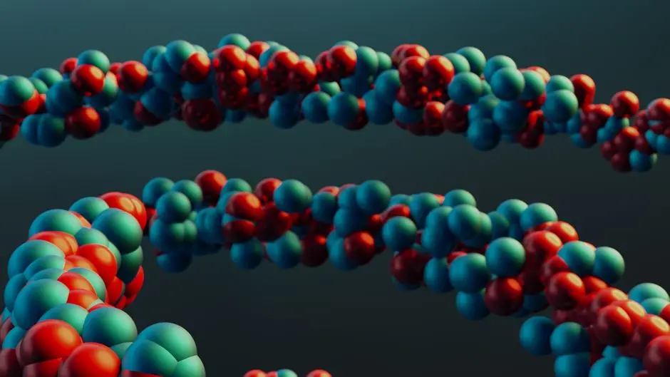
Unlock the profound power of protein language models and their generated embeddings to revolutionize biological discovery. Understanding how to precisely compare these intricate vector representations is not merely a technical exercise; it is a critical leverage point in modern bio-engineering. We activate a new era of research where functional inference, novel enzyme discovery, and rational drug design are driven by data-centric methodologies. The ability to quantify the resemblance between protein embeddings empowers us to navigate vast biological spaces, identifying relationships previously obscured by sequence-level analysis.
This article guides you through the essential Python approaches for measuring similarity between protein embeddings, transforming abstract concepts into actionable computational strategies. We reveal how to select, implement, and optimize the metrics that drive breakthroughs. Prepare to master the tools that harness the transformative power of AI and Transformers for protein sequence modeling, empowering your pursuit of biological frontiers.
Decode Protein Embeddings: The Foundation for Comparison
We embark on this journey by first establishing a robust understanding of protein embeddings. These numerical vectors serve as high-dimensional, semantic representations of proteins, capturing complex structural, functional, and evolutionary information. Traditional sequence alignment struggles to capture distant evolutionary relationships or subtle functional nuances; embeddings transcend these limitations by mapping proteins into a continuous vector space where proximity implies biological relatedness. Each protein sequence, processed by advanced language models, transforms into a dense vector, its dimensions encoding intricate features like secondary structure propensities, domain interactions, or ligand binding sites.
The fundamental premise for comparing these embeddings is the geometric interpretation of their relationships in this vector space. When two protein embeddings reside close to each other, their corresponding proteins share significant biological attributes. Our objective is to precisely quantify this 'closeness.' This foundational step – transforming raw sequence data into meaningful, comparable vectors – is the crucible where bioinformatics meets machine learning, activating a powerful new paradigm for protein analysis. We acknowledge that the quality of these embeddings directly impacts the validity of our similarity assessments, underscoring the importance of selecting robust pre-trained models or meticulously fine-tuning custom architectures. This initial setup lays the groundwork for all subsequent comparisons, ensuring we operate on rich, informative data.
# Python setup: We activate the necessary libraries for our exploration.
import numpy as np
from sklearn.preprocessing import normalize

# Forge dummy protein embeddings for demonstration.
# In a real pipeline, these would originate from a protein language model
# (e.g., ESM-2, ProtT5, AlphaFold-Embeddings).
# Each row represents a protein embedding; each column is a dimension.
# We engineer 3 embeddings, each with 128 dimensions.
protein_embedding_A = np.random.rand(1, 128) # Protein A embedding
protein_embedding_B = np.random.rand(1, 128) # Protein B embedding
protein_embedding_C = np.random.rand(1, 128) # Protein C embedding

# Let's create a small dataset of embeddings to simulate a collection of proteins.
# We will use this array for subsequent similarity calculations.
embeddings_matrix = np.vstack([protein_embedding_A, protein_embedding_B, protein_embedding_C])

print("Generated protein_embedding_A shape:", protein_embedding_A.shape)
print("Generated embeddings_matrix shape:", embeddings_matrix.shape)
print("\nFirst 5 dimensions of protein_embedding_A (sample):", protein_embedding_A[0, :5])
Quantify Resemblance: Euclidean Distance and Cosine Similarity
We now engage with the two bedrock metrics for quantifying protein embedding resemblance: Euclidean Distance and Cosine Similarity. Each offers a distinct perspective on 'closeness' in our high-dimensional space. Euclidean Distance, the intuitive 'straight-line' distance, measures the absolute magnitude of difference between two vectors. A smaller Euclidean distance signals greater similarity. However, this metric is sensitive to the magnitude of the embedding vectors; if some embeddings have significantly larger norms due to their generation process, Euclidean distance can be misleading. We must always consider whether raw magnitude variation is biologically meaningful or merely an artifact.
Conversely, Cosine Similarity focuses on the angle between two vectors, effectively measuring the similarity of their directions, irrespective of their magnitudes. A cosine similarity close to 1 indicates that the vectors point in nearly the same direction, signifying high similarity. Values near 0 suggest orthogonality (no linear relationship), and -1 indicates opposite directions. Cosine similarity excels when the absolute scale of the embeddings is less important than their directional orientation, a common scenario in semantic similarity tasks. We engineer our approach by understanding that selecting the appropriate metric is not arbitrary; it depends on the inherent properties of the embeddings and the biological question we aim to answer. For instance, if embedding magnitude encodes a specific biological feature like protein size or abundance, Euclidean distance might be more appropriate. Otherwise, cosine similarity often provides a more robust measure of functional or structural relatedness, especially after L2 normalization.
# We activate Python's numerical prowess for precise similarity calculations.
from scipy.spatial.distance import euclidean, cosine

# Let's assume we want to compare protein_embedding_A and protein_embedding_B
# Ensure embeddings are flattened for direct distance/similarity functions if they are 2D (1, N)
emb_A = protein_embedding_A.flatten()
emb_B = protein_embedding_B.flatten()
emb_C = protein_embedding_C.flatten()

print("\n--- Euclidean Distance --- ")
# 1. Forge Euclidean Distance: Measures the straight-line distance between two points in Euclidean space.
# Lower values indicate higher similarity.
euclidean_dist_AB = euclidean(emb_A, emb_B)
euclidean_dist_AC = euclidean(emb_A, emb_C)
print(f"Euclidean Distance between A and B: {euclidean_dist_AB:.4f}")
print(f"Euclidean Distance between A and C: {euclidean_dist_AC:.4f}")

print("\n--- Cosine Similarity --- ")
# 2. Forge Cosine Similarity: Measures the cosine of the angle between two vectors.
# Values range from -1 (opposite) to 1 (identical direction). Higher values indicate higher similarity.
# Note: scipy's cosine function returns cosine *distance*, so we subtract from 1 to get similarity.
cosine_sim_AB = 1 - cosine(emb_A, emb_B)
cosine_sim_AC = 1 - cosine(emb_A, emb_C)
print(f"Cosine Similarity between A and B: {cosine_sim_AB:.4f}")
print(f"Cosine Similarity between A and C: {cosine_sim_AC:.4f}")

# Insider Tip: For robustness, we often normalize embeddings before cosine similarity,
# although cosine itself inherently focuses on direction.
# Let's demonstrate explicit normalization and re-calculate.
emb_A_norm = normalize(emb_A.reshape(1, -1), axis=1).flatten()
emb_B_norm = normalize(emb_B.reshape(1, -1), axis=1).flatten()

cosine_sim_AB_norm = 1 - cosine(emb_A_norm, emb_B_norm)
print(f"Cosine Similarity (normalized) between A and B: {cosine_sim_AB_norm:.4f}")
Beyond Basic Proximity: Advanced Similarity Approaches
Our exploration extends beyond Euclidean and Cosine, delving into additional similarity metrics that offer nuanced perspectives. Manhattan Distance (or Cityblock Distance) computes the sum of the absolute differences of their coordinates. This metric finds its leverage when movement along dimensions is constrained or when the 'cost' of dissimilarity adds up linearly across features. In contrast, Chebyshev Distance (or L<sub>∞</sub> distance) identifies the maximum absolute difference across any single dimension. This proves invaluable when the largest deviation in any one feature dictates the overall perceived dissimilarity, often relevant in error-sensitive applications.
We confront the 'curse of dimensionality' – a pervasive challenge where the efficacy of distance metrics diminishes in very high-dimensional spaces. In such scenarios, all points tend to appear equidistant, obscuring true relationships. To mitigate this, we employ Dimensionality Reduction techniques like Principal Component Analysis (PCA) or Uniform Manifold Approximation and Projection (UMAP). PCA linearly transforms data to a lower-dimensional space, preserving variance and revealing primary drivers of variation. UMAP, a non-linear method, excels at preserving local and global data structure, often yielding visually insightful clusters. Applying these techniques before similarity computation can distill signal from noise, improve computational efficiency, and reveal latent biological organizations. We engineer our pipelines to strategically leverage these methods, ensuring that our similarity assessments remain robust and biologically relevant even when confronted with complex, high-dimensional embedding spaces.
# We activate further computational tools to explore advanced similarity concepts.
from scipy.spatial.distance import cityblock, chebyshev
from sklearn.decomposition import PCA
import matplotlib.pyplot as plt

# Let's generate a slightly larger set of dummy embeddings for PCA demonstration
np.random.seed(42) # Ensure reproducibility
dummy_embeddings = np.random.rand(50, 128) # 50 proteins, 128 dimensions

# Forge Manhattan (Cityblock) Distance: Sum of absolute differences along each dimension.
# Useful when movement along axes is restricted or cost is additive.
emb_A = dummy_embeddings[0]
emb_B = dummy_embeddings[1]

manhattan_dist_AB = cityblock(emb_A, emb_B)
print(f"\nManhattan Distance between A and B: {manhattan_dist_AB:.4f}")

# Forge Chebyshev Distance: Maximum absolute difference along any single dimension.
# Useful when one dimension's difference dominates the perception of dissimilarity.
chebyshev_dist_AB = chebyshev(emb_A, emb_B)
print(f"Chebyshev Distance between A and B: {chebyshev_dist_AB:.4f}")

print("\n--- Dimensionality Reduction for Visualization and Noise Reduction ---")
# Optimize embeddings by reducing dimensionality using PCA.
# This can help mitigate the 'curse of dimensionality' and reveal underlying structures.
# We select 2 components for visualization.
pca = PCA(n_components=2)
reduced_embeddings = pca.fit_transform(dummy_embeddings)

print(f"Original embeddings shape: {dummy_embeddings.shape}")
print(f"Reduced embeddings shape (PCA to 2D): {reduced_embeddings.shape}")

# Visualize the reduced embeddings (conceptual).
# This code snippet would typically be part of a larger plotting script.
# We just print a sample to show the transformation.
print("First 5 reduced embeddings (PCA):\n", reduced_embeddings[:5])

# plt.figure(figsize=(8, 6))
# plt.scatter(reduced_embeddings[:, 0], reduced_embeddings[:, 1], alpha=0.7)
# plt.title('Protein Embeddings Reduced to 2D with PCA')
# plt.xlabel('Principal Component 1')
# plt.ylabel('Principal Component 2')
# plt.grid(True)
# plt.show()
Engineer Scalable Search: Approximate Nearest Neighbors (ANN)
When confronting datasets comprising millions or even billions of protein embeddings, traditional brute-force similarity calculations become computationally intractable. We engineer a solution: Approximate Nearest Neighbors (ANN) algorithms. These powerful methods drastically reduce search time by sacrificing a minuscule amount of accuracy, delivering results that are 'good enough' for most biological discovery pipelines. Libraries like Facebook AI Similarity Search (FAISS), Annoy, and HNSW (Hierarchical Navigable Small World) implement various ANN strategies.
FAISS, in particular, offers a robust framework for managing vast embedding spaces. It operates by building an index that partitions the high-dimensional space, allowing queries to efficiently locate neighbors without comparing against every single item. Key to FAISS is the concept of `IndexIVFFlat`, where embeddings are quantized into clusters. During a query, only a subset of these clusters (defined by `n_probe`) are searched, providing a substantial speedup. This approach introduces a critical trade-off: increasing `n_probe` improves search recall (finding more true nearest neighbors) but prolongs query time. We optimize our ANN pipelines by meticulously balancing speed and accuracy, a decision driven by the specific demands of the biological application. Activating ANN transforms computationally expensive similarity tasks into real-time discovery engines, allowing us to rapidly screen vast protein libraries for candidates with desired properties, from drug targets to novel biocatalysts. This is the cornerstone of scalable bio-engineering, forging pathways to accelerate scientific progress.
# We engineer a scalable similarity search pipeline using FAISS.
import faiss
import time

# Prepare a larger dataset of dummy embeddings to simulate a real-world scenario.
# Forge 10,000 protein embeddings, each with 128 dimensions.
np.random.seed(42)
dataset_embeddings = np.random.rand(10000, 128).astype('float32') # FAISS requires float32
query_embedding = np.random.rand(1, 128).astype('float32') # Our query protein

d = dataset_embeddings.shape[1] # Dimension of embeddings
n_data = dataset_embeddings.shape[0] # Number of items in the dataset
n_probe = 10 # Number of clusters to search (for IVF index)

print(f"Dataset size: {n_data} embeddings, dimension: {d}")

# --- Traditional Brute-Force Search (for comparison) ---
start_time = time.time()
# Calculate all pairwise distances (e.g., using cosine similarity, inverted as distance)
# For simplicity here, we'll just demonstrate the brute force concept conceptually.
# In reality, this would involve a loop or matrix operation to find the closest.
# For a single query, we would iterate through all dataset_embeddings and calculate similarity.

# Example of brute-force Euclidean distance for a single query (slow for large datasets)
# distances = np.array([euclidean(query_embedding.flatten(), emb.flatten()) for emb in dataset_embeddings])
# nearest_idx_brute = np.argmin(distances)
# print(f"Brute-force search took: {time.time() - start_time:.4f} seconds")


# --- Forge FAISS Index for Approximate Nearest Neighbors (ANN) ---
print("\nForging FAISS Index...")

# Step 1: Choose an index type. We activate an `IndexFlatL2` for exact L2 (Euclidean) search first.
# This is often a good baseline, but not approximate.
# index_flat = faiss.IndexFlatL2(d)
# index_flat.add(dataset_embeddings)

# For approximate search, we activate an `IndexIVFFlat` (Inverted File Index with Flat quantizer).
# This index quantizes vectors into 'nlist' clusters and then searches only relevant clusters.
nlist = 100 # Number of clusters.
quantizer = faiss.IndexFlatL2(d) # The base index for storing vectors within each cluster
index = faiss.IndexIVFFlat(quantizer, d, nlist, faiss.METRIC_L2)

# Train the index (this step is crucial for IVF indexes).
# The training process learns the cluster centroids.
start_time = time.time()
index.train(dataset_embeddings)
print(f"FAISS Index training took: {time.time() - start_time:.4f} seconds")

# Add the embeddings to the trained index.
start_time = time.time()
index.add(dataset_embeddings)
print(f"FAISS Index adding embeddings took: {time.time() - start_time:.4f} seconds")

# Set the number of probes for search (how many clusters to check).
index.nprobe = n_probe # Higher n_probe means better accuracy but slower search.

# Perform a similarity search for the query embedding.
# We seek the top 5 most similar proteins (k=5).
k = 5
start_time = time.time()
distances, indices = index.search(query_embedding, k)
print(f"FAISS Search for top {k} took: {time.time() - start_time:.4f} seconds")

print(f"\nTop {k} similar protein indices (FAISS): {indices.flatten()}")
print(f"Corresponding distances (FAISS): {distances.flatten()}")

# Insider Tip: Evaluate recall. For production, activate rigorous testing to balance speed vs. accuracy.
# For example, compare FAISS results against a small brute-force calculation on a subset.
Activate Insights: Interpreting and Applying Embedding Similarity
Our journey culminates in the most critical phase: activating biological insights from the quantitative similarity scores we have meticulously calculated. A numerical value, whether a high cosine similarity or a low Euclidean distance, holds little intrinsic meaning until we translate it into biological context. We interpret high similarity scores (e.g., cosine similarity >0.9) as strong indicators of functional or structural homology, suggesting shared protein families, conserved active sites, or similar molecular mechanisms. Moderate scores (e.g., 0.7-0.9) might reveal broader evolutionary relationships, shared domains, or nuanced functional variations, prompting deeper investigation into specific sub-families or divergent activities.
We apply these insights across a spectrum of bio-engineering challenges. In functional annotation, we leverage similarity to assign putative functions to novel proteins, accelerating the understanding of newly sequenced genomes. For drug discovery, identifying proteins similar to known drug targets can uncover potential off-target effects or suggest repurposing strategies. We optimize enzyme engineering by locating natural enzymes with similar active site architectures, providing templates for rational design or directed evolution. Furthermore, embedding similarity guides de novo protein design, allowing us to validate computational designs against natural protein space or identify regions with desired characteristics. A crucial insider tip: always activate critical thinking. Embedding similarity provides powerful hypotheses, but experimental validation remains paramount. Over-reliance on computational similarity without experimental confirmation constitutes a common pitfall. We forge ahead, using these computational tools as potent compasses to navigate and conquer the complex frontiers of biological discovery, ensuring each insight propels us closer to impactful breakthroughs.
# No new code for this section, as it focuses on interpretation and application.
# However, we reinforce the output interpretation from previous steps.

# Recall: Our similarity scores (e.g., cosine similarity of 0.85, Euclidean distance of 0.5).
# We now activate the critical step of translating these numbers into biological meaning.

# Scenario Example:
# Let's say we compared a query protein (unknown function) to a database of known proteins.
# The FAISS search returned:
#   - Top 1 protein: Index 1234, Cosine Similarity: 0.95 (Highly similar)
#   - Top 2 protein: Index 5678, Cosine Similarity: 0.88 (Moderately similar)
#   - Top 3 protein: Index 9012, Cosine Similarity: 0.75 (Lower similarity, but still related)

# Interpretation Checkpoints:
# 1. High Cosine Similarity (>0.9): Often indicates strong functional conservation,
#    similar structural folds, or shared protein families.
# 2. Moderate Cosine Similarity (0.7-0.9): Suggests broader evolutionary relationships,
#    shared domains, or functional sub-types.
# 3. Low Cosine Similarity (<0.7): May point to distant relationships or
#    novel functions that need deeper investigation.

# Biological Leverage Points from Similarity:
# - Functional Annotation: Assigning function to unknown proteins based on similar known proteins.
# - Drug Discovery: Identifying proteins similar to known drug targets for repurposing,
#   or identifying off-target effects.
# - Enzyme Engineering: Discovering novel enzymes with specific desired catalytic activities
#   by searching for similar active sites or overall protein architectures.
# - Protein Design: Guiding de novo protein design by identifying regions or features
#   of natural proteins that achieve specific biological outcomes.

print("\n--- Activating Biological Insights from Similarity Scores ---")
print("A cosine similarity of 0.95 between an unknown protein and a known enzyme often strongly indicates functional homology.")
print("Conversely, a lower score, while indicating less direct similarity, might pinpoint a novel variant or a protein with a modified function, requiring experimental validation.")
print("We must always remember that these scores are computational predictions; experimental validation remains paramount to confirm biological hypotheses.")
Key Takeaways
Protein Embeddings: The New Biological Language
Protein embeddings transform complex protein sequences into high-dimensional numerical vectors, capturing intricate functional, structural, and evolutionary relationships. These representations empower us to move beyond basic sequence alignments, revealing deeper biological insights through quantitative comparisons in a continuous vector space. Quality embeddings are foundational for accurate similarity assessments.
Core Similarity Metrics: Euclidean vs. Cosine
We deploy two primary metrics: Euclidean Distance measures the absolute straight-line separation, sensitive to vector magnitude. Cosine Similarity quantifies the angle between vectors, focusing on directional agreement irrespective of magnitude. We choose the appropriate metric based on whether the absolute scale of embeddings or their directional orientation holds greater biological significance for the specific analysis.
Advanced Techniques for Robust Comparison
Beyond basic metrics, we leverage Manhattan and Chebyshev Distances for nuanced perspectives on feature-wise differences. To combat the 'curse of dimensionality' and distill meaningful signals, we strategically apply Dimensionality Reduction techniques like PCA or UMAP, enhancing the clarity and interpretability of embedding relationships in high-dimensional spaces.
Scaling Discovery: Approximate Nearest Neighbors (ANN)
For vast protein datasets, we engineer scalable solutions using Approximate Nearest Neighbors (ANN) algorithms, such as those provided by FAISS. These methods drastically accelerate similarity searches by trading minimal accuracy for significant speed gains. We optimize ANN pipelines by balancing recall and query time, enabling real-time discovery in large protein libraries.
Biological Activation: Interpreting and Applying Scores
The ultimate goal is to activate biological insights from numerical similarity scores. High scores often indicate strong functional or structural homology, while moderate scores suggest broader relationships. We apply these insights to functional annotation, drug discovery, enzyme engineering, and protein design. Crucially, all computational predictions require experimental validation to confirm biological hypotheses and avoid common pitfalls.
FAQ
-
Why use protein embeddings instead of traditional sequence alignment for similarity?
We utilize protein embeddings because they transcend the limitations of sequence alignment. While alignment focuses on direct sequence homology, embeddings capture high-level semantic, structural, and functional information, even for evolutionarily distant proteins with low sequence identity. They represent proteins in a continuous vector space where proximity signifies deep biological relatedness, providing a more robust and scalable approach for complex biological queries.
-
Which similarity metric should I choose for my protein embeddings?
The choice of similarity metric depends on your biological question. We select Cosine Similarity when the direction of the vector (semantic content) is more critical than its magnitude, often suitable for functional or structural comparisons. We deploy Euclidean Distance when the absolute difference and magnitude are biologically meaningful. Consider Manhattan or Chebyshev Distance for specific scenarios where feature-wise differences are paramount. Always validate the chosen metric against known biological relationships in your specific domain.
-
How do I handle very large protein embedding datasets for similarity search?
For large datasets, we engineer our pipelines with Approximate Nearest Neighbors (ANN) algorithms. Tools like FAISS, Annoy, or HNSW allow us to conduct rapid similarity searches by creating an index that efficiently queries relevant subsets of the data, rather than performing computationally expensive brute-force comparisons. We optimize ANN search by balancing the trade-off between search speed and recall accuracy.
-
What are common pitfalls when comparing protein embeddings?
We identify several common pitfalls. First, ensure the embeddings are generated from a model appropriate for your task; low-quality embeddings yield unreliable comparisons. Second, be wary of the 'curse of dimensionality' in very high-dimensional spaces, which can make all points appear equally distant – dimensionality reduction can mitigate this. Third, never interpret similarity scores in isolation; always contextualize them with known biological data and validate findings experimentally. Fourth, improper normalization can skew distance metrics. We activate rigorous testing and biological validation to circumvent these errors.
-
How can I interpret the biological meaning of a similarity score?
We interpret a high similarity score as a strong indicator of shared biological properties, such as functional conservation, structural 유사성 (similarity), or membership in the same protein family. A lower, but still significant, score might suggest broader evolutionary links or shared domains. We activate the biological context of the proteins involved and existing domain knowledge to translate numerical scores into actionable biological hypotheses. Always remember that these are computational predictions that demand experimental validation for conclusive biological insight.